Configuring Rendering Lighting¶

For instructions on how to run these tutorial notebooks, please see the index. This tutorial, in particular, would benefit from running locally; it relies heavily on OpenGl implementations and the Drake website publishing pipeline does not have a graphics card. So, you may prefer running it locally.

tl;dr¶

This tutorial is about controlling the illumination in your rendered scenes. The goal is to give you proper intuition and techniques for efficiently and effectively lighting your scenarios. The goal is to end up with renderings like this (rendered in the final section of this tutorial):

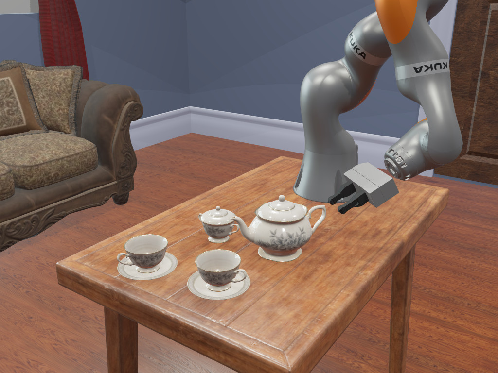Figure: Example of a rendering using RenderEngineVtk PBR rendering.

The discussion is limited to a single rendering technology: physically-based rendering (PBR). This is available when using RenderEngineVtk. RenderEngineVtk also has a legacy Phong illumination model (also used by RenderEngineGl). This tutorial will not discuss the Phong illumination model. If curious, we recommend further reading on Wikipedia.

Tutorial Overview

• Overview of rendering model (PBR)
• Tutorial methodology and infrastructure
• Direct lighting
  • Shadows
• Materials
• Environment maps
  • Tone mapping and exposure
• Total illumination
• Putting it all together

Physically-based Rendering (PBR)¶

An illumination model is an approximation of the physics behind the physical phenomena underlying vision -- electromagnetic radiation strikes materials and reflects towards a photo-sensitive medium (e.g., film, CCDs, human eyes, etc.) The so-called "physically-based rendering" illumination model is a modern model that hews more closely to actual physics (in comparison with older, classical illumination models). While it is truer to reality, it is still an approximation. There will inevitably be differences between renderings and reality.

What makes it physical?¶

PBR's primary distinction is that it returns to the underlying physics of light:

• It's based on a statistical model of how light interacts with materials at a microscopic level.
• It conserves energy.

PBR provides concrete benefits:

• It allows content authors to create models based on an object's actual properties without concern about how the objects get used; the correctness of the material doesn't depend on the lighting.
• Simply put, it produces more realistic images.

To effectively light a scene, you need to understand the properties of the available light sources and how materials respond to those light sources. For example, if you have an object painted with Vantablack shining more light on the object will not appreciably change your final image. This tutorial provides a high-level discussion of the material properties and light sources available to you. If you're interested about the details of PBR, you might try this tutorial or this documentation of a particular implementation.

Enabling PBR in RenderEngineVtk¶

The discussions below will be interleaved with interactive examples where you can explore the parameters discussed. We'll simply start with how to enable PBR illumination.

RenderEngineVtk defaults to the Phong illumination model for historical reasons. This default will change in the future. In the meantime, there are three things that will change a RenderEngineVtk instance from Phong to PBR:

• Explicitly request it in the RenderEngineVtkParams
  • Set the force_to_pbr flag to true.
• Add an environment map.
• Add at least one glTF file (Drake's preferred visual geometry representation) to the RenderEngineVtk instance. More specifically, add a drake::geometry::Mesh with drake::geometry::PerceptionProperties compatible with your RenderEngineVtk instance.

Tutorial methodology and infrastructure¶

Methodology¶

As we discuss the details of PBR and Drake, we'll do it in a context in which you can explore the parameter space.

In addition to the code blocks in which you can modify parameters and re-evaluate, we've given you the ability to move the camera and re-render the image. We'll do that via an instance of meshcat visualizer. By moving the camera in the visualization browser window, the camera in this session will update its pose to match. It does require explicitly re-rendering.

Each render will print the command for setting the camera pose. If you change the camera to something you like and would like to consistently reproduce it, you can copy and paste the command into the render window.

The pattern you'll see over and over again is a pair of code blocks. The first will set up the scene -- with particular emphasis on the parameters being illustrated. It also sets a curated camera pose so that the first rendering you do will show what the tutorial needs to show.

The second code block will simply perform the rendering (and contain the rendered result). The first evaluation will use the camera pose defined in the first block. Subsequent executions of the rendering block will use the pose from the meshcat session.

To streamline the first code block, we'll introduce some infrastructure to admit compact declarations of scenes.

Infrastructure¶

The necessary imports.

We'll create a special system that will track the camera position in the meshcat session.

Now, we'll create the RenderComparator class. This class will allow us to instantiate multiple renderers for a single scene. When we render from the comparator, each of the render engines will render a color image, and the comparator will display the array of images.

It also gives us short-cuts for populating the scene with simple primitives.

The first rendering¶

Let's test the infrastructure. We'll see if we can render a simple image.

We'll also start a meshcat instance here. It is typical to do this once at the beginning of the notebook, and use the same instance throughout.

In order to be able to track the camera's position in the Meshcat session, you must open the modified url (the one that ends with ?tracked_camera=on) which will print out after executing the next block.

Once meshcat is up and connected, this block will check to make sure that camera tracking is properly enabled. If it fails but you're sure that meshcat is up and running on the correct URL, simply re-evaluate it again until it reports success.

Set up the render framework¶

The block below is the first block which sets up the rendering. In this first rendering, we'll instantiate the comparator, populate it with some geometry, push the geometry to meshcat, configure a RenderEngine, and, finally, pose the camera.

For subsequent renderings, we may not do all of these (for example, several renderings in a row can use the same geometry).

Invoke rendering¶

In the meshcat visualizer, you should now see a white sphere on a grey plane (well, large, flat box). Evaluating the next block should render an image of the same scene and display that image below the code block.

The first rendering is from the camera pose defined above. Subsequent invocations of render() will pull the pose from meshcat visualizer. Each time you render, make note of the output comparator.pose_camera_once(...) associated with the image. That is the pose command that you can use to reproduce the image shown.

Try changing the view in your meshcat session and re-evaluating the next block. Confirm that the render perspective changes with the visualizer's view. If not, confirm the block above, testing the camera feedback, prints out "Camera tracking enabled!"

Practice manipulating the view. You'll probably be doing that a fair amount during the course of this tutorial.

ATTENTION: Expect the rendered image to deviate from what is shown in the meshcat browser. Meshcat introduces an independent light set from those defined in the RenderEngine. Meshcat also uses a PBR illumination model, so much of what is described for RenderEngineVtk will also apply there although the exact details will differ.

The default light¶

If no lights are specified (see below), there is a default light: a single light affixed to the camera. That is why the ball always looks the same, regardless of how the camera moves. The light is always shining straight ahead from the camera. However, the ground plane's level of illumination does change based on the viewing angle.

Direct Lighting¶

You can think of virtual lights as objects that emit light energy in rays. The direction of the rays plays a significant role in how the objects in your scene get illuminated (see below). Basically, the various light types vary in the definition of those light rays.

In this section, we'll focus on the distribution of light in the scene from each light type. We won't focus too much on specific reflection effects (that requires an understanding of materials).

Drake supports three kinds of lights: point, spot, and directional.

• Point light: This is essentially an idealized light bulb. It has zero radius so all light rays emanate from a single point, parameterized by drake::geometry::render::LightParameter::position. The rays are emitted in all directions. Defining the light's position determines the emitted light rays' common origin and directions.
• Spot light: This is a point light with an opaque, conical light shade on it, parameterized by drake::geometry::render::LightParameter's fields: position, direction, and cone_angle. Like a point light, it emits all light from a single point (located at position). However, there is an oriented cone associated with the spot light. The cone has its apex at position and it expands in the direction indicated by the direction vector. Finally, the cone_angle controls how narrow the spot light's beam is. The angle (in degrees) specifies the half angle of the cone's span, or the angle between the cone's central axis and the boundary of the cone. No light is emitted outside of this cone.
• Directional light: This can be thought of as a point light that is infinitely far away, or idealized sunlight; all emitted light rays are parallel. As such, the directional light has no meaningful value for position, but its direction value defines the direction of the emitted light rays.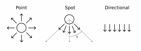

Figure: The three kinds of explicit lights.

Computing diffuse illumination¶

Light interacts with matter in various ways. While the physics is fascinating and intricate, rendering technology typically focuses on the effects and creates algorithms that approximate many of the observable effects. The names you might see in this regard are such things as: "diffuse", "specular", "ambient", "reflection", "refraction", "diffraction", etc., This tutorial won't necessarily discuss all supported phenomenon. Instead, it will touch (and possibly elaborate) on those lighting effects that are most relevant to exploring the rendering configuration.

Diffuse lighting¶

When light strikes a surfaces, some portion of the light is reflected off of the surface and some portion is refracted into the surface. The light that refracts into the surface may bounce around several times before bouncing out again.The bouncing is a random process. Even though a light ray may strike a surface from a specific direction, the final refracted light can end up shining in an arbitrary direction. Thus, from a viewer's perspective, the observed refracted light doesn't depend on which direction the light ray came from, but simply how much light struck the surface. Furthermore, the light color and intensity can be changed by this process (as some frequencies of light get filtered out and energy gets absorbed as part of the bouncing around).

To fully account for this refracting phenomenon, we need to add up all of the light that can strike that surface point from any direction (this is, in fact, a hemisphere of directions; light rays coming from "behind" the surface point do not illuminate it). As we sum up all of the light sources and account for the energy loss and color shifts, we end up with the total refracted light emitted from the point on the surface.

This process "diffuses" the lighting shining onto the surface, blurring, tinting, and dimming it from the viewer's perspective. (Note: we'll discuss the reflected portion down below when we talk about "specular" reflections.)

The question of "how much light" strikes the surface is affected by the intensity of the light sources and the angle at which the light ray strikes the surface. A light ray striking the surface perpendicularly will have the most energy. As the angle becomes shallower, the amount of light striking the surface will get smaller. This is computed based on the normal of the illuminated surface and the direction of light rays produced by each light type.

For a scene with a flat plane, we can see the different diffuse lighting effects that the three lights have. We'll render a flat plane with three different lights: a point light 5 meters above the plane, and a spot light 5 meters above the plane, shining straight down, and a directional light shining directly down on the plane.

So, let's look at the distribution of light from each light type.

Don't forget, repeated executions will render from your meshcat camera perspective.

There are some essential differences between the three images. Let's look at those differences and see how light choice effects them.

The most obvious difference is the spot light's limit. It doesn't illuminate the full ground box. We see a circular pool of light. The light is circular because the spot light's cone of light intersects the ground perpendicularly. If the spot light were tilted, the pool of light would be elliptical. In RenderEngineVtk, the spot light's pool of light always has a hard edge.

A more subtle difference is between the point light and directional light images. In both images, the ball's appearance is essentially the same. However, the ground box is different. With the point light, the ground nearest the ball is the most brightly illuminated. Away from the ball, the ground is much darker. In contrast, the ground box is the same color everywhere with the directional light. It's also worth pointing out that within the pool of light, the spot light's pattern of illumination matches the point light. Why is the directional light different?

In order for a surface to be visible (to eye or camera), light must strike the surface. The more light that strikes it, the brighter the surface appears. Three light properties determine the amount of light striking the surface: direction, intensity and attenuation.

Direction¶

For a beam of light with a fixed energy level, the portion of that energy that actually reflects off a surface depends on the angle at which the beam strikes the surface. If the light strikes the surface perpendicular to the surface, the energy (per unit area) is maximized. As the beam's approach direction diverges from perpendicular, less energy per unit area strikes the surface, so there's less to reflect. The surface will appear dimmer. As the light direction becomes parallel to the surface, the surface will not be illuminated at all. Obviously, any light beam coming from behind an opaque surface will not illuminate it all.

So, how does that apply to the images above?

The point light and directional light (and spot light, of course) have the same intensity. The point light is placed above the ball so that light striking the top of the ball strikes the ball perpendicularly. Similarly, the directional light is aimed straight down. That is why the ball in both images appears more or less identical.

However, as we consider the ground far away from the ball, the relationship between surface orientation and light direction differs. By definition, the rays from the directional light are the same throughout the whole scene. That's why the ground has constant illumination across its visible surface. However, the direction from surface to point light changes as we move away from the center; less light is striking those areas because of the shallower angle.

Try changing the direction of the directional light or the position of the point light in the previous rendering to see how illumination levels change.

Intensity¶

Intensity is simple to understand. It is simply how much energy is in the electromagnetic radiation. In LightParameter, the intensity controls this energy level (see below). As the light intensity increases, the amount of energy reaching the camera can exceed the camera's ability to display. Details are lost as the pixels saturate to white. Too little intensity, and the image becomes an indistinguishable black blob.

Attenuation¶

In the real world, light intensity decreases as the distance to the light increases. This attenuation of physical light follows the inverse-squared law -- if distance doubles, intensity falls to a quarter. The lights above have no attenuation. The distance to the light has no bearing on light intensity. For truly realistic scene lighting, we should change the lights to have quadratic attenuation.

LightParameter also includes attenuation parameters. It is a triple of coefficients: (c, l, q). A light's intensity gets attenuated based on the distance, d, between light source and illuminated point. The scale factor is:

total_attenuation = 1 / (c + l * d + q * d²)

The inverse-squared law is satisfied by c = 0, l = 0, q = 1. In practice, it sometimes becomes convenient to have the intensity decay more slowly by reintroducing constant or linear factors. The sum of the three coefficients should total one. If the sum is less than one, light intensity will get boosted. If all three coefficients are zero, the light has infinite intensity.

Note: Attenuation does not apply to directional lights as there is no concept of "distance" with those lights.

Combining lights¶

A scene can include multiple lights. Sometimes, it is necessary to use multiple lights to create the final effect of real-world lighting. For RenderEngineVtk you can declare as many lights as you like, although more lights mean greater computational cost.

Shadows¶

Note: This section in particular would benefit from running locally. The website images have numerous shadow artifacts (e.g., splotches of shadow appearing on illuminated surfaces).

None of the previous renderings had any shadows. Everything was illuminated as if there were nothing between the surface and the light. In the real world, light can be occluded. Physical objects block the light, casting shadows onto surfaces that would otherwise have been lit. In rendering, we don't get occlusion for free. We create shadows through a variety of approximations. The spot light's cone of light is our first example. In the real world, that cone of light is created by a physical shade that blocks emitted light. The virtual spot light is simply modeled as a cone of light directly. However, this simplified cone model, while sufficient for creating a pool of light, is insufficient for shadows.

There are multiple techniques to detect occlusion. RenderEngineVtk uses a technique called "shadow maps". Shadow maps are an encoding of surfaces that are visible to the light source. Any surface that is visible gets illuminated. Surfaces that are not visible are in shadow. A shadow map is a texture map (hence the name), where every pixel contains a value storing the distance of the closest surface in the direction of the pixel. These distance measurements are reconciled at rendering time to determine if a surface is in shadow or not.

This shadow model is binary. A pixel is either visible from the light or not (up to possible numerical precision issues). Given that our lights are all modeled as point sources (more or less), this binary illumination classification means that all shadows will have hard edges; there is no blurry penumbra.

Let's explore these phenomena. But first, let's make sure shadows work.

You should clearly see that the ball casts a shadow on the ground plane in the image on the left. The image on the right is a repeat from before, but has explicitly disabled shadow casting. If you see the shadow, you can proceed with the next steps to see how the various settings control the shadow appearance.

(Keen observers will no doubt notice the pixely edge of the shadow. That topic is explored below in the "Shadow resolution" section.)

What lights can cast shadows?¶

Spot lights and directional lights can cast shadows. Point lights cannot. This is not a fundamental property of the model, but one of how RenderEngineVtk is implemented. We'll get a bit more into the implementation details and how they relate to this when we consider the limitations on spot light shadows below.

The following renderings will enable shadows and each uses a unique light type. Notice that we've changed the light position (bringing the spot and point lights closer to the ball).

As promised, the point light casts no shadow on the ground plane. Declaring cast_shadows = True is not an error for point lights; the value simply has no effect. Conversely, the spot and directional lights both cast shadows, there are some obvious differences between the shadows.

• The shadow cast from the directional light is smaller than that of the spot light. Not only that, it even appears smaller than the ball.
  • The directional shadow is definitely smaller than the spot light shadow. Because the spot light's light rays diverge, the shadow will be larger than the object casting it. This is illustrated in the figure below in the shadow map resolution section.
  • However, the directional shadow is not smaller than the ball itself. This is an optical illusion due to perspective. The ball's shadow is, in fact, the same size as the ball itself. But the shadow is farther from the camera than the ball itself. And in perspective, the closer something is, the larger it appears. Try moving the camera and re-rendering. When the camera is close to the ground, it is clear that the shadow has the same radius as the ball.
• The spot light's shadow has a much smoother edge than the directional light. The directional light's shadow has a clearly pixelated edge. This is due to shadow map resolution (see below).

As a side note, the lighting levels on the ball from the directional light is now quite different from that of the point and spot lights. We moved the point and spot lights closer to the ball. So, the surface normal direction and direction to light deviates more quickly along the surface of the ball, changing the effect of the lighting. If we were to move the spot and point lights farther from the sphere, the effect would quickly become indistinguishable from the directional light.

Spot light limitations¶

While spot lights can cast shadows, their ability is limited by the cone half-angle (the cone_angle parameter). It can cast shadows with a cone_angle value up to 90 degrees. The following renderings show how a too-large cone_angle eliminates shadows.

We get a ball shadow for the 50- and 85-degree spot lights. The 90-degree spot light casts no shadow.

The reason for this is related to RenderEngineVtk's implementation. It is the same reason that point lights cast no shadows. The entire space visible to the light is mapped to a single 2D image via a simple projection. If every possible shadow a light can cast projects onto a single plane, then that light can cast shadows. This is true for a spot light with cone_angle < 90 degrees. The plane whose surface normal is parallel with the light's directional vector can catch all of the shadows. But once the cone_angle value reaches 90-degrees, there are emitted light rays that are parallel to that plane. They will never intersect with the plane and therefore can't cast shadows onto it. In RenderEngineVtk, shadows are simply disabled for such spot lights.

The second thing to note about the images is that the quality of the shadows. The shadows from the 50-degree spot light and the 85-degree spot light are obviously different. The shadow from the 85-degree spot light has been reduced to a single, slightly blurry rectangle. This is a good time to get into shadow map resolution.

Shadow map resolution¶

The shadow map is a rendering of the scene from the camera's perspective. Each pixel stores the distance from camera to the nearest surface in the direction of the pixel. This makes it closely resemble a depth map. The following illustration shows a simple scene with a sphere and box being illuminated by a spot light.

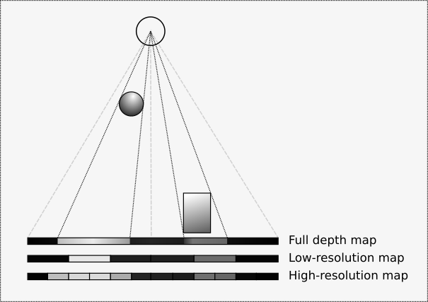Figure: Shadow map resolution: the resolution of the shadow map will determine how much detail is present in the shadow. Too little resolution, and the blocky shadow map pixels become apparent in the final rendering.

Below the scene are visualizations of possible shadow maps, each with different resolution. The "Full depth map" represents the idealized shadow map. In this case, we've colored "far" values as black and "near" values as white. Note that although the sphere is smaller than the box, because it is closer to the spot light, it has a larger footprint in the shadow map. This idealized map doesn't have pixels, per se.

The next row down shows a coarse approximation of the idealized map. In this case, the domain of the shadow map has been reduced to six pixels. The coarse sampling leads to significant aliasing issues. The extents of the sphere and box in the shadow map have changed significantly. It is easy to imagine that for a 3D scene, the shadow of the sphere will be turned into a single square pixel, just as we observed above from the 85-degree spotlight.

The final row doubles the resolution over the previous row. There are still sampling artifacts, but the approximation of the actual shadow boundaries has definitely improved.

Warning: There is a cost for each shadow-casting light. The scene must be rendered once for each light at each frame to create that light's up-to-date shadow map. The more lights that cast shadows, the more times the scene has to be rendered to produce one output image.

Let's look at the RenderEngineVtkParams::shadow_map_size parameter and see its impact on the shadows.

For a fixed light, we can easily change the shadow map resolution to improve the visual fidelity of the shadow edges. But this is a setting that needs to be used judiciously. It would be "safe" to simply set all shadow maps to some large (power-of-two) value to make sure that shadows all look clean. However, this comes at a cost. Each shadow map must be re-rendered with each frame. The speed of this depends on the rendering capability of your computer. It might be reasonable to try setting shadow map resolution high straight across the board and see if the performance is appreciably harmed. But, generally, the best strategy is to use the lowest resolution map that provides a visually acceptable shadow.

Shadow map registration¶

It is one thing to define the resolution of the image that stores the shadow map. But what is the relationship of that image and the rendered world? In other words, how big are those pixels? The bigger the pixels, the more likely you are to notice the resolution.

The shadow map has to be "registered" to the world in some way -- defining which portion of the world is accounted for by the shadow map. The image is finite, the world is, in principle, infinite. So, only some portion of the world can be included in the domain of the shadow map. There are no parameters for controlling this domain of shadow coverage. So, how is it defined?

Both shadow-casting lights have their domains automatically and dynamically computed on every rendering. At their core, each light determines the extent of those objects that can be illuminated by the light, and registers the shadow map to cover that full domain.

This domain is updated on a render-by-render basis to prevent objects moving in and out of regimes in which shadows can be cast. However, it means if the extent of the scene changes significantly from render to render, the shadows may qualitatively change as well (e.g., previously smooth shadows become blocky).

Each shadow-casting light uses its own proprietary logic for determining the illuminated domain.

Spot light registration¶

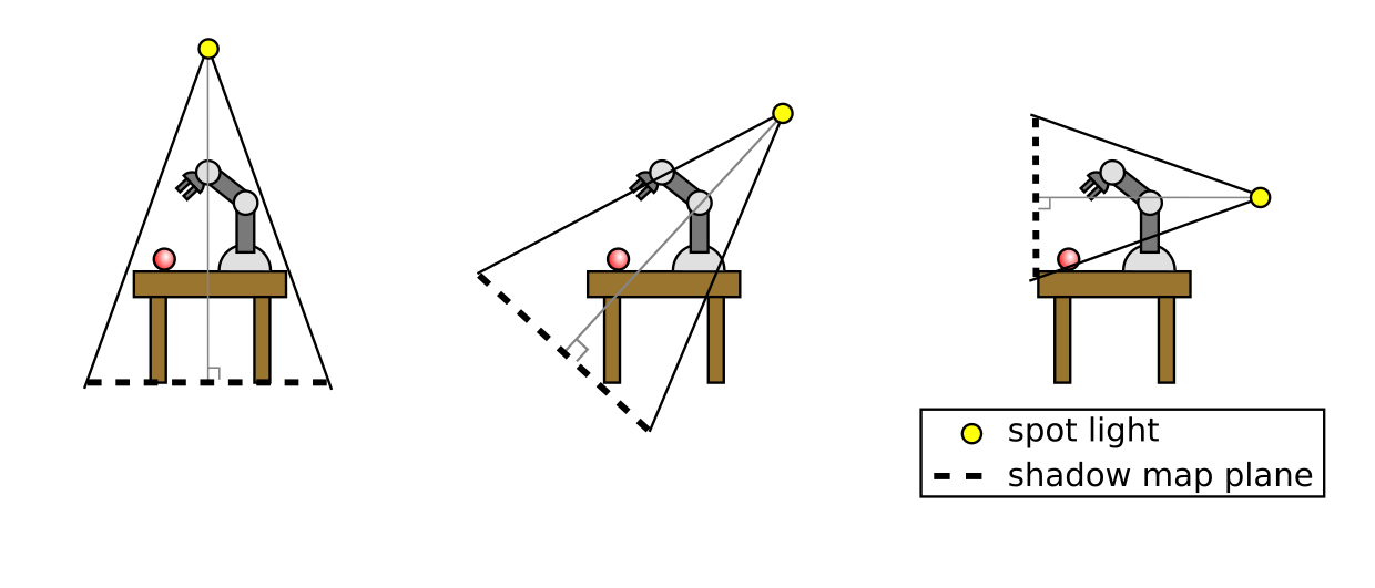
The spot light determines the domain of its shadow map (its light volume) by creating a view frustum. The frustum is oriented so that the near and far planes are perpendicular to the light's direction vector. The planes are scaled so that the cover the extent of the cone; the frustum is tapered towards the source. The near plane is directly in front of the light source itself. The far plane is moved away from the light's position in the light direction until it as far as the farthest scene element in that direction.

Implications

1. No matter how "deep" the scene is in the direction of the camera's view, the shadow pixels at any depth will be the same size as the size of the pixels largely only depends on the cone angle of the light. So, simply fixing cone angle and then modifying the map resolution size will define the pixelation on the shadow boundaries.
2. If the scene is "deep" in the direction of the camera's view, but we're only rendering the items nearest the camera, we will effectively have reduced precision in the depth calculations. This only affects thin objects piled on top of each other.

Directional light registration¶

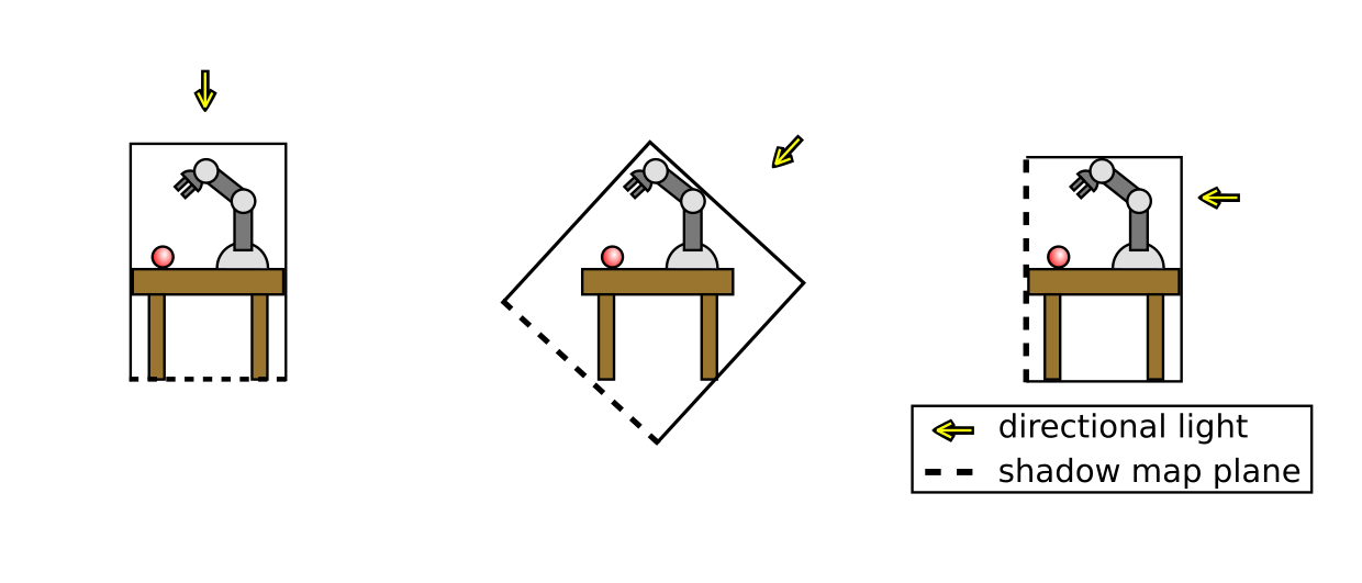
Directional lights don't have finite extent. They can, in principle, cast light anywhere in the world. In this case, the extent of the illuminated domain is defined by the extent of the geometry that can be illuminated. Essentially, we create a bounding cube around all of the geometry aligned to the light's direction vector. The size of the cube face is the size of the shadow map in the world.

Implications

1. The more the scene spreads out perpendicular to the light's direction, the more shadow map resolution you need. Rendering scenes with ground planes can cause the shadow volume to increase to enclose a volume much larger than the subject of the camera. This will require much higher shadow map resolution to get a good effect near the subject, wasting much of the shadow map resolution.
2. If the shadow map gets "stretched" out because of the scene bound, it may be that enabling shadows will produce no discernible effect. It may simply be that the shadow map has been stretched so large, that a shadow map pixel is larger than your target objects; they simply don't render into the shadow map.

Let's see what that looks like.

Given that the light is emitting parallel light rays perpendicularly into the ground, we would expect the ball's shadow to be the same size as the ball itself. It is. Given the focal length of our render camera, we're getting strong perspective effects -- things farther from the camera are scaled smaller than things closer. When the ball is closer to the camera than its shadow, it will appear larger. When the shadow is closer to the camera than the ball, the shadow will appear bigger. The important thing to note is that these shadows are both expected and correct.

PBR Materials¶

The previous section was all about controlling a source of light (not the only source of light, more on that later). However, emitting light is only the start. We're interested in how it reflects off of surfaces to the camera. To understand that, we need to talk about how materials are modeled in the PBR model. If you have the wrong model in your mind, you might be surprised why changing light properties doesn't have the effect you expect.

Again, this discussion is going to be heavily biased towards intuition and principle. Visit one of the links in the introduction to get into the fine details of the material definitions.

Microfacts and reflections¶

We see specular reflections every day. These are the mirror-like reflections such that images of the environment are visible on the surface. Even some of the most non-mirror-like surfaces exhibit some degree of specular reflection -- dull concrete surfaces will still show highlights when you look at it from the right angle. Take a look at this site to see how even the "dullest" objects have specular reflections.

The physics of these reflections is conceptually simple. Light strikes a point on a surface (with an associated surface normal). The incoming light ray is reflected across the normal. If your eye is on the path of the outgoing ray, you see the reflected light. Another way of saying the same thing is to imagine the "half-angle vector" between the incoming light direction and the outgoing view direction. If that vector is aligned with the surface normal, you see a reflection.

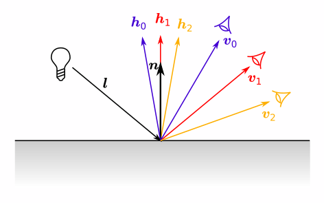Figure: The light ray strikes the surface with normal n from direction l. The three views v₀, v₁, and v₂ form half-angle vectors h₀, h₁, and h₂, respectively. Only h₁ aligns with n, so only view v₁ receives the specular reflection from the light source.

In the real world, surface reflectivity can vary widely. Some crisp and clear and others so subtle that you have to look carefully to notice it. These differences come down to the structure of the object surface at a microscopic level.

No surface is perfectly smooth. At the microscopic level, irregularities in the material produce many different normals within a small region. As light strikes that region, light will get distributed in many directions simultaneously, based on the distribution of face normal directions. Shiny surfaces are more regular in structure. The majority of microfacets face the same way. Dull surfaces have more chaotic structure. The more coherency in microfacet direction there exists, the shinier the surface and the more distinct the reflection.

The effect of this is twofold. First, perceived specular reflections from a highly irregular surface are both dimmer and blurrier. Dimmer, because the light from a single direction gets scattered in multiple directions simultaneously; only a small portion of the incoming light energy from a single direction gets reflected in the viewer's direction. Blurrier, because the light that does get reflected in the viewer's direction can come from a larger span of angles.

PBR takes a statistical approach to accounting for these microfacets. A single rendered pixel may encompass millions of microfacets. So, in PBR, we describe a surface's "roughness". At any given point on the surface, there is an attendant roughness value. From this roughness value, we can determine what portion of the microfacets are aligned with the half-angle vector, h. Let's see what that looks like.

As roughness increases, the specular reflection of the light grows larger (i.e. blurrier) and dimmer. This is consistent with PBR's goal to conserve energy.

Clarifications on specular reflections¶

1. The light sources described above are all, in some sense, point lights. As the surface gets smoother (roughness going to zero), the reflection becomes a more exact reflection. Mathematically, when roughness is zero, the specular reflection of light sources are mathematical points. These points would not appear in the rendering; the measure of the point is infinitely small. This is correct, with respect to the PBR model, but counterintuitive when modeling the physical world. When computing the specular reflection from direct light sources, Drake makes sure the specular highlight does not completely disappear.
2. The lighting model does not include specular reflections of one geometry in the surface of another. Getting mirrored surfaces that reflect other geometry requires a different kind of technique -- one that RenderEngineVtk does not support yet. So, the only specular reflections we will see are those from scene artifacts that are considered to be light sources, e.g., the explicit lights described above and the environment maps described below.
3. Specular reflections always depend on three things: the direction the light ray comes from when striking the surface, the orientation of the surface (its normal direction), and the direction from the surface to the camera.
4. When light strikes a surface at a "grazing" angle, the surface exhibits greater reflectivity (called Fresnel reflections).

Diffuse illumination and "metallness"¶

Specular reflections come from the light that bounces off a surface. However, not all light reflects off. Some light refracts into the surface. Depending on the material, some of the light bounces around inside a bit, getting filtered by the material, and bounces out again. This is what makes the surface visible away from areas of perfect specular reflections.

In contrast to specular reflections, the diffuse illumination does not depend on the direction from surface to viewer. Diffuse illumination only depends on the available light sources and the surface's normal.

PBR models two kinds of materials: metallic and dielectric. Metallic materials are, as the name implies, made of metal. Dielectric materials are, more or less, all other non-metallic materials (e.g., plastic, concrete, wood, glass, etc.).

These two materials behave very differently with respect to the light.

• metallic
  • Metallic materials absorb all refracted light. That means that they don't exhibit any diffuse reflection. Away from specular reflections, they are essentially not illuminated.
  • Specular reflections get heavily tinted by the metal's intrinsic color (its "albedo"). If you look at gold, copper, etc., you'll see the reflections in those materials have been tinted to the metal's underlying color.
• dielectric
  • Dielectric materials exhibit diffuse reflection. Light does escape from the surface away from the specular reflections.
  • Specular reflections tend to be dimmer than with metallic materials (the ratio of how much light gets reflected vs. refracted is much lower). Furthermore, the reflections are not tinted by the material's albedo.

Although, both metallic and dielectric surfaces can display Fresnel reflections, the effect is typically more noticeable on dielectric materials, because their base reflectivity is generally much lower than that of metals.

In PBR, these two properties are modeled using a "metallic" property ("metallicFactor" in glTF files). In principle, this should be a binary value; a surface is either metallic or dielectric. However, due to interpolation in texture look up, the model handles all values between zero and one, even if it's not physically meaningful to say a material is halfway between being metallic and dielectric.

Let's look at these material differences in play.

The two spheres are strikingly different. They both have the same albedo (underyling color) and roughness values. All of the differences are attributable to the difference between metallic and dielectric.

Obviously, the metallic sphere is quite dark, almost like it isn't being illuminated at all. This is the result of two things we've discussed. Metallic surfaces only exhibit specular reflections (never diffuse), and the only scene artifacts that participate in the specular reflections are light sources; we won't see the dielectric sphere reflected in the metallic sphere.

Second, the specular reflection of the light itself differs across the two spheres. The metallic sphere's "hot spot" is larger and somewhat oversaturated in the center (we'll deal with the oversaturation when we discuss exposure later). Again, this is because the metallic surface reflects a larger portion of the incoming light than the dielectric surface, so more radiant energy reaches the eye.

Finally, the highlight on the metallic surface has a gold tint to it, one that the dielectric's highlight is missing. This is the metallic surface refracting all of the non-gold light frequencies internally.

Try varying the roughness to see how each material type changes. Things get particularly interesting when roughness goes to one.

We'll explore some more differences again in the next section: environment maps.

Environment Maps¶

The name "environment map" probably invites an intuitive interpretation: a painted backdrop. Rather than modeling an entire environment, we simply put an image in the background which we can see directly and reflected in mirror-like surfaces. While that's true, it's not the whole story. An environment map is a light source. That means it will participate in specular reflections. But it will also participate in diffuse reflections as well. Essentially, each pixel in the environment map is a light source (more on this later).

We'll start with a simple environment map and a mirror ball.

The image below shows a ball in a simple environment. The mirror ball sits on a gray plane. Around it are three rectangular area lights. Blue and red lights on either side and a brighter white light above it.

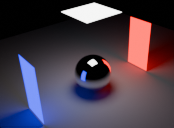Figure: The physical environment.

We can make an environment map by replacing the mirror ball with a panoramic camera. The panoramic image defines what is visible around a point in all directions. Essentially, we're painting on the inside of an infinitely large sphere. But we do so with a rectangular image. The mapping between the rectangular image and the sphere is an equirectangular projection. The height of a pixel spans a fixed solid angle of the sphere. The width of a pixel spans the larget solid angle at the "equator" of the image (central, horizontal line). But the width of the pixels get smaller as you near the top and bottom of the image (or north and south poles of the sphere). We'll make use of this when we attempt to predict the lighting contribution of the environment map.

Figure: The environment map drawn from the physical scene shown above.

The red and blue lights are easily identified in the image. The top of the image is the single white area light above the camera. In a Mercator projection, the north pole gets spread across the full width of the top of the image. The light directly above the camera has received the same treatment.

The environment should also have appeared in your meshcat session. Rotate the camera to see the various light panels. (The image is quite low resolution, so the light panels should appear as blurry rectangles.) Ultimately, the full effect of the environment map will be easier to understand when applied to a scene.

For the next few scenarios, we're going to disable direct light sources entirely and only look at the effect of the environment map. If you haven't done so already, you should turn off Meshcat's lights by opening the "Controls" window an unchecking the blue box next to "Lights". This will bring the Meshcat window's version closer in line with the renderings in this tutorial.

We'll use the previous set of gold-ish balls and see the effect the environment map has on it.

The metallic sphere is no longer black with a hot spot (as it was with the single direct point light). This is because the environment map provides light in every direction, giving the metal surface something to reflect. Again, all of the reflections have been tinted the metal's gold-ish albedo color.

Similarly, the dielectric sphere is reflecting the environment. The specular reflections are dimmer and untinted as before. But there are some other things going on as well.

Note: the total light level in meshcat will appear brighter than in the rendered image. This is directly attributable to the fact that we're using a png image (the same would happen with jpg and other so-called "normalized color" image types). VTK and meshcat handle the mapping of such images into environment maps slightly differently, leading to a difference in illumination levels. Reducing the //Render Settings/<object> exposure value to around 0.35 will approximately unify the images. When using high-dynamic range images (see below), the differences essentially go away and tweaking exposure will not be necessary.

Let's try tweaking the exposure.

Now, let's take a closer look at how the environment map interacts with dielectric materials.

This time we've put the camera between the two spheres and the red light in the environment map. We can still clearly see the specular reflection of the white light and the red light in the smooth sphere on the left. The rough sphere on the right has no such specular reflection.

But this image illustrates two additional phenomena: Fresnel reflections and diffuse illumination.

The Fresnel reflection is apparent in the smooth sphere. We can see the blue light reflected on the rim of the smooth sphere. The fact that the sphere reflects the blue light is expected. But the fact that the reflection of the blue light is more intense than the white or red lights might be surprising. The light striking the surface at a grazing angle experiences greater reflectivity so we observe a more intense reflection.

Both spheres have a reddish tint that covers a large portion of the side of the sphere. If you move the camera in Meshcat to look at the blue sides of the spheres and re-render, you'll see a similar blue tint on the other side. This is the environment map's contribution to the diffuse lighting effects.

Remember, diffuse illumination is the portion of radiant energy that comes from the portion of the light that strikes the surface, refracts inwards, bounces around and, finally is partially emitted again. The total diffuse effect is the sum of all such light. If there's a light source from any direction that can strike a point on the surface, it must be included in the diffuse calculation.

In this case, for any given point on the sphere, half of the environment map is able to shine light onto the sphere (it is the hemisphere of the environment centered on the point and arrayed around the surface normal at that point). Because of the integral and the energy-conserving properties of the PBR model, the total contribution of the environment map on the diffuse lighting is a blurred and dimmed version of the environment.

This effect can also be thought of as a form of "ambient" lighting. When light is shined into a room, the light doesn't simply leave the light source and strike a single surface before bouncing to your eye. The light bounces many, many times. With each bounce the reflected light can change in character. Light simply moves so fast that we can't observe this phenomenon; we merely see the steady state of the light having bounced everywhere. This is the reason why surfaces can be illuminated even if the light source can't shine directly onto the surface; there is "indirect" lighting that does shine onto it. This indirect lighting is the "ambient" light of the environment.

High-Dynamic Range (HDR) Images¶

Not all images can serve equally well as environment maps. A typical image -- one typically seen as part of a webpage -- uses "normalized" color. That means the value for each pixel is a value in the range [0, 1] (or [0, 255] depending on encoding). The environment map above uses just such an image. Normalized color is sufficient for communicating basic color information (hue, saturation, etc.) but it has limited ability to communicate the full dynamic range of radiant energy possible. While physical light has varying frequency (signalling color in our minds), it also has intensity. An ideal environment map is one that can encode both color and intensity. High-dynamic range (HDR) images use unnormalized color data. They still communicate color properties (again, hue, saturation, etc.), but they also encode intensity. The range between the dimmest and brightest portions of the environment map can be arbitrarily large (as it is in most human environments). We frequently don't notice the wide range of intensities because our eyes and brains are good at taking a wide range of light levels and creating a coherent image in a narrow range of energy levels. Cameras typically have a smaller dynamic range than the human optical system, so photographers are always worrying about shutter speed, film speed, and aperture to control how much light energy the image medium is exposed to.

This is of critical importance when it comes to curating environment maps. Environment maps encoded in normalized color images (e.g., png, jpg, bmp, etc.) will have a different impact on the rendering than an unnormalized color image (.hdr). In an environment map, a light intensity is associated with each pixel. Light intensity can be characterized with various units. We'll use watts (W) as being reasonably correlated with the brightness of the light. For a normalized image, the maximum energy at every pixel, regardless of color, is 1 W (pure white pixels); colors with less value (darker colors) implicitly have less energy with pure black being the only zero-energy pixel. To put that in context, in real world scenarios, intensity can range multiple orders of magnitude between the darkest and brightest light sources. That has two implications for normalized color images:

• The maximum intensity of 1 W is quite dim compared to the real world.
• They provide almost no lighting contrast. What contrast exists usually comes from the colors in the image and the general correlation with low intensity light sources manifesting as dark colors to film and sensors. As counter-intuitive as it might seem, a pixel with dark normalized color (0.01, 0.01, 0.01) is putting out 1 W of light, just like a white pixel. It's just 1 W of essentially "black" light (but not in the "all-night rave" sense of the word).

Each environment map encodes a certain amount of radiant energy. Let's take a look at the impact the difference in energy can have.

To that end, we'll use three different environment maps which only differ in how much irradiant energy they inject in the scene. All three maps represent the same abstract environment shown above (with the red, blue, and white area lights). They have the same resolution and color information at each pixel.

• PNG: a normalized image with brightness of 1 W.
  • The irradiant energy is limited by the file format itself.
• 7.5 HDR: an HDR image with maximum brightness of 7.5 W.
  • The irradiant energy in the environment map was controlled by specifying the power of the corresponding lights in the scene. The brightest light was a 7.5-watt light.
• 120 HDR: an HDR image with maximum brightness of 120 W.
  • The power of all lights in the 7.5-watt scene were multiplied by a constant factor of 16 (making the brightest light 120 Watts).

For the next few experiments, we'll create a small matrix of spheres. Horizontally, we'll vary smoothness, and vertically we'll vary material (metallic vs dielectric).

Although the three images use environment maps with the exact same resolution and the same color values at every pixel, the differences in pixel energy produce significantly different results.

The 1-watt .png image is both dim and has low contrast (for the reasons suggested above). The 7.5-watt image contains a larger range of illumination and leads to a more vibrant image with greater contrast. The image rendered with the 120-watt image takes this even further. So far, in fact that the image has become oversaturated and the three of the four balls have all but disappeared.

Just as we can take a direct light and increase its intensity so much that the rendered image becomes painfully oversaturated, environment maps can do the same.

(The appearance of the background is also changing. But, instead of getting lighter like the foreground elements, it's getting darker. We'll look into that in the next section.)

The rendered images clearly depend significantly on the light levels in the environment maps. Does this mean that there are some environment maps that are simply unusable? They have too much energy? Good news! We are free to use any environment map; we just need to control how the camera's "film" is affected by the light.

Meshcat can make use of the same environment maps, leading to similar outcomes. Execute the following blocks to change Meshcat's environment map. As with the renderings above, you should see a similar effect (in terms of increased brightness and contrast).

Tone mapping and exposure¶

We need to take a brief detour to understand how high dynamic range images get drawn to your screen (and saved as normalized color images).

In the images above, the image using the 1-watt .png image has 1/120th the light energy as the image rendered with the 120-watt environment map. And yet, the "dim" image is not simply a copy of the bright image with each pixel having 1/120th the value of the original. If that were the case, the image would just be near-black silhouettes of the balls against a black background. However, the balls are not silhouettes. There is still visible gradation of light communicating the rounded shape of the balls. In fact, the dim, 1-watt image shows more of the spherical shape for the bottom row of balls than the oversaturated 120-watt image. So, what's happening?

The answer is "tone mapping". It's the process by which an image with "unbounded" intensity levels gets mapped to an image (or display) with normalized color. The mapping is not strictly linear. Generally, near the darkest and brightest features, there is non-linear tapering in attempt to preserve details at the extremes of illumination. Furthermore, as the images show above, the tone mapping function has a finite range -- intensity values outside of that range produce the saturated white pixels we've seen in some of the previous images.

There are, in fact, various possible mapping functions. RenderEngineVtk uses the "Generic Filmic tone mapping operator with the "Uncharted2" parameter values. There are multiple parameters associated with that operator. To keep things simple, Drake exposes a single parameter: exposure. If you are familiar with photography, exposure plays a similar role in rendering as it does in photography. It is essentially a way to control how much the "film" is exposed to the the scene's radiant energy. Expose it less and the final image is darker. Expose it more, and the image is brighter. Go too far in either direction, and the final image can either be a dark mess or a washed out blur of whiteness. In RenderEngineVtk, exposure is simply a scale factor applied to the image prior to performing the non-linear mapping. So, if a pixel in the resulting image is reflecting 10 W to the camera, an exposure value of 0.5 will mean we map a 5-watt intensity at that pixel. The default value for exposure is 1. Images that are too dark should increase exposure and images that are too bright should reduce exposure.

It's clear in the above image that the image using the 1-watt .png image is underexposed (three of the four balls are obviously underlit). At the same time, the image using the 120-watt .hdr image is overexposed. Let's render the images again, but this time tune the exposure.

The exposure values below, have been selected so that the top of the rough, dielectric sphere basically appears the same in all images. (We'll come back to the question of how do you pick exposure values later.)

We can see the effect of exposure on the three images. In all three cases, the top of the rough dielectric ball appears about the same.

While the target ball in the 1-watt image now resembles the ball in the 7.5-watt image, the other balls and background have changed significantly. What happened? In this case, it's because the "dark" area of the environment map is not true black. There is a non-zero amount of illumination which has been scaled by a factor of 7.5, pushing it far enough from black that when the subsequent tone mapping is applied, "black" has become medium grey. This illustrates an important principle. If the lighting levels lie within a narrow range, exposure may not be sufficient to increase contrast.

The target ball in the 120-watt image has been pulled back to the same grey as the 7.5-watt image. It is no longer over saturated and the curvature of the ball can easily be seen. However, the black in the mirror ball is darker than the mirror ball in the 7.5-watt image. This is because the 120-watt image has a larger range. However, the grey background in the 7.5-watt and 120-watt images has the same energy level. But in the 120-watt image, that amount is much smaller compared to the maximum intensity. So, when tone mapping is applied, that background intensity is functionally black and renders as such.

Judicious use of exposure is critical in producing images that are both aesthetically pleasing as well as modeling sensors which also are sensitive to exposure. That said, remember we've currently only exposed a single parameter related to tone mapping. In the future, we may expose more parameters if exposure proves to be insufficient on its own.

Meshcat is not necessarily using the same tone mapping function, but it uses one and has, likewise, exposed its exposure value. It can be found in the Control under the RenderSettings/<object> tabs. The exposure value defaults to 1 and has a similar effect in Meshcat as the value does for RenderEngineVtk. For example, the following block sets the environment and controls the exposure.

Where do you get environment maps?¶

The two easiest ways to get environment maps are from downloading or creating.

Open source environment maps can be downloaded from repositories like Polyhaven.

The simple environment maps used in this tutorial were created in Blender. There are copious tutorials on Youtube on how to do this, like this one.

Total Illumination¶

Environment maps can't cast shadows. Direct lights can. A fully-lit scene can include both.

Getting them to work together can be tricky. It's easy to configure lighting with both environment map and direct lights such that one of the two lighting sources has no apparent effect.

This typically arises if there is a significant difference between the energy levels of the direct lights and the environment map.

To get shadows and the benefit of the environment map, it is necessary to balance the direct light intensity with the environment. (Failing to do so would be like trying to use a flashlight to cast shadows outdoors on a sunny day.)

The images below use a fixed exposure, an environment map, and a downward-pointing spot light. The scenes differ in the spot light's intensity. At low intensity, the effect of the light is almost negligible. As the light's intensity increases, the effect of the light becomes apparent and we get effective shadows. As the light becomes too powerful, the image becomes oversaturated.

As we did before with oversaturated images, we'll use exposure to reduce the oversaturation effects. And, as before, we'll use the illumination of the rough dielectric ball as the guide for choosing the exposure. In this case, we disabled the shadows while determining those values (as the shadows interfere with our lighting rubric).

In all five images, the rough dielectric balls are basically the same. This has understandably led to attendant changes in the other balls.

There are multiple important lessons to draw from the images above.

Balance: The images with the 0.1-watt and 100-watt lights show massive imbalance between the direct lights and the environment map. In the 0.1-watt image, the spot light has almost no effect (only the faintest of shadows can be seen below the spheres). In the 100-watt image, the light outshines the environment map by so much, that the perfect specular reflections in the smooth metallic ball have been almost entirely eliminated by the tone mapping. The fundamentally dimmer specular reflections in the smooth dielectric ball have been eliminated.

In contrast, the 1-watt and 2-watt (and even the 7.5-watt) images show a better balance between direct illumination and environment map.

Materials: The mirror ball is not just perfectly smooth (roughness = 0), but it is also metallic. Metallic materials are unaffected by diffuse light effects, including from the environment map. The appearance of metallic surfaces are dominated by specular reflection.

If the material were non-metallic instead, in addition to the specular reflection attributable to its smoothness, it would also be illuminated by the diffuse and ambient lights.

However, the two rough spheres (on the right) appear similar. If metallic balls don't get diffuse light, how is the rough metallic sphere so brightly illuminated? Does the roughness somehow cause diffuse lighting effects? No. It is still only specular reflection, but the roughness has caused the reflection to become so blurred, that it has a diffusive-effect. What you'll notice if you move the camera, is that the appearance of the rough metallic ball will change as the camera moves, whereas the rough dielectric ball remains unchanged.

Exposure values: The baseline image uses an image consistently described in this tutorial as having a "7.5-watt white light". And yet, when we add a 1-watt or 2-watt light to the scene, we have to reduce the exposure to 0.55 and 0.4, respectively. And when we add a 7.5-watt spot light, the exposure drops all the way down to 0.11 all in the name of normalizing the appearance of the top of the rough sphere.

Previously, we said that the exposure is simply a scale factor on the surface's reflected radiant energy. If the environment map has a 7.5-watt top light and we add another 7.5-watt direct light, why would we have to reduce the exposure to ten percent of its original value and not simply half? Conversely, by adding a 1-watt or 2-wat light, we reduced the exposure to around half which implies that the intensity of the environment on the top of the ball was approximately 1-2 W.

We discussed that the diffuse illumination contributed by the environment map is the result of finding the average light over the hemisphere associated with the surface point and normal. The hemisphere is large and the white light is small (speaking as solid angles). Therefore, the diffuse intensity is significantly lower than the peak intensity in some portion of the hemisphere. If the white light were larger, spanning a larger solid angle, more energy would bleed out as diffuse illumination. In this case, averaging the red, white, and blue light sources with the dark background produces a peak diffuse intensity of only about 1-2 watts from the environment map.

This means you can't determine compatible intensities for direct lights just by looking at the peak intensities in the environment map.

So, how do you pick intensity values for your lighting? For now, tinkering.

Putting it all together¶

Let's go ahead and apply all of that in lighting a scene.

We'll build up a scene of something more interesting than spheres and then we'll iterate on the lighting in the scene.

First, let's populate the world with a table, a robot arm, and a tea set.

Let's get ready to render.

• We're going to change the camera a bit. Rather than using Meshcat's camera, we'll more closely approximate a 35-mm lens by changing the focal length.
• We'll add a default RenderEngineVtk. It will automatically be in PBR mode because all of the models we're adding are glTF files.

• Finally, we'll pick an initial camera pose so we can see what's happening.

  Evaluating the next block may print a warning. You can ignore it. Drake's models include texture optimizations for Meshcat that VTK ignores. We may see that same warning each time after we call comparator.set_render_engines().

Now let's render it.

We can clearly see the table with the robot arm and tea set on top. The gripper appears to be reaching for the teapot's handle. We made no explicit declarations about the lighting, so we have the default "headlamp" light for RenderEngineVtk.

The background color is quite light and the scene objects appear relatively dark. For now, we won't worry about the background color (we'll address that later). But let's tweak the exposure so that we can make out the objects in our scene better. The exposure value used below is completely subjective; we picked a value such that we liked the rendered result more than the other values we sampled.

Note: Again, there is a difference between the VTK and Meshcat images. The Meshcat image is more brighly illuminated. More particularly, the robot, table, and dishes are all tinted by the background color. The reason for this is that Meshcat uses the background as an environment map, even when none is provided. In this case, the scene is embedded in a cloud that casts pale blue light on it from all directions. If you edit the background colors (//Background/<object>) you will see an immediate impact on the illumination of the scene. Don't worry about the difference, it will go away as soon as we apply an HDR image as an environment map.

The scene objects are now much easier to see.

It's a good starting point, but we don't necessarily want the objects floating in the clouds. So, let's give it an environment. Using models available through Drake's model repository, we've put together a simple environment and rendered it into an environment map. This is like what we did above to create our toy environment map, but this time, it's a bit more interesting.

Let's load the environment and take a look.

The room has four lights on the ceiling and a window open to the daytime sky. The light coming through the window is brighter than that from the light bulbs.

Take a look at the environment map in the meshcat visualizer to get a better view of the room.

Now let's apply the environment map to the scene.

Note: we're not rendering the environment map in the background (skybox=False). There are several notable differences between the images:

• Reducing the exposure has unsurprisingly caused the background color to get darker.
• There are clearly more apparent light sources; you can see multiple highlights on the robot arm.
• Despite the reduced exposure, the table is more brightly illuminated in this image than it is in the previous image. This is due to several reasons:
  • In the previous image, the camera is facing forward in the camera view, so the light direction is moving mostly across the table surface instead of down onto it. In contrast, the environment map has multiple lights shining from above the table.
  • The intensity of the lights in the environment map are greater than the single default headlamp.
• The light positions are independent of the camera position. That means much of the robot arm appears darker because it's no longer being illuminated directly from the camera position.
  • In fact, if you turn the camera in meshcat to look at the scene from the window's side, you'll be able to see the window's contribution to the scene.

The addition of the environment map is a definite improvement over the default light.

Let's see what it looks like when we render the environment map.

The foggy background is now gone. Try moving the meshcat camera and re-render the scene. Try some of the following angles:

• Look at the table across from the window (so that you can see the window in the rendering).
• Do the same, but face the room's door.
• Look from the perspective of the window.

In two of those views, the background seems to be overly dark. However, when looking at the robot arm and the window in the same rendering, the background and scene elements seem far more well balanced. Why is that?

It's primarily due to the light intensity. Before we apply tone mapping (via the exposure parameter), we first collect the amount of light energy at each pixel. When we put the camera at the window and look at the table, we see the window's full light contribution reflecting off the scene's objects. Behind those objects, however, we have a wall which contributes very little light in comparison. Therefore, when we apply the tone mapping, the brightest part of the image (the foreground elements) look just right, and the background gets pushed closer to black.

When we look at the table with the window behind the table, both the window's light energy and the highlights on the table, robot, etc. have a similar intensity. So, they get treated in a very similar way by the tone mapping process.

This is an inherent problem with environment maps. Their true purpose is to serve as a source of lighting to the objects in the scene. Also using it as a backdrop in the scene may not have the desired result. So, what can be done?

The simplest solution is to actually put in a background; objects that can actually reflect the same light as the foreground elements.

Let's reload the scene, but this time, we'll add the geometry of the room as well.

The inclusion of the background geometry has two immediate impacts:

• There is something to reflect the same light that the robot is; the background is lighter than when we were simply using the environment map as a backdrop.
• The perspective on the background is correct.
  • Environment maps treat the environment like it's infinitely far away from the illuminated objects.
  • In this case, that's a very poor approximation of the environment; the room's walls are just a few meters away from the foreground elements. When the camera moves away from the center of the environment's center, what is shown in the background is increasingly incorrect. By including geometry for the environment, it maintains the correct spatial relationship as the camera moves.

Note There is currently a known defect in RenderEngineVtk; transparent objects are not rendered properly. So, when you turn the camera to look across the robot into the window, it is no longer brightly illuminated; the window is treated as opaque.

Because the environment map correlates with the room geometry, we're getting great specular and diffuse effects which really tie the geometry in with the rest of the room. Let's see if we can get some shadows.

When adding lights, we advocate the following process:

1. Pull the camera back so you can actually see what you're doing.
2. Add one light at a time.
3. When adding a light, make sure it's the only light source.
4. Set the light intensity incredibly high so you can see its effect. This will help getting the posing of the light right; you want to easily see where the light is being cast.
5. Disable shadows; an occluded light provides very few clues on why it isn't contributing.
6. After the pose is confirmed:
   • Enable shadows.
   • Reintroduce other light sources.
   • Tune the new light's properties to work with the existing set.

So, let's do that. Let's attempt to create shadows from the open window. In this case, we know the window lies in the -Wz direction from the robot arm. So, we're going to start the light shining in the +Wy direction. We'll simply run through a number of iterations in sequence without discussion (beyond code comments).

So, now we have some subtle shadows coming in from the window. Let's see if we can't get shadows from the four lights in the ceiling. Applying the same process as above, we arrive at the following. Feel free to try the same process above to determine your own configuration for the ceiling lights.

The shadows are subtle. They become more apparent when objects are in motion. Sometimes it can be easy to be fooled by a single image.

Here are a couple more curated viewpoints to look at the scene.