A guide to using hydroelastic contact in practice.
Introduction
There are many ways to model contact between rigid bodies. Drake uses an approach we call “compliant” contact. In compliant contact, nominally rigid bodies are allowed to penetrate slightly, as if the rigid body had a slightly deformable layer, but whose compression has no appreciable effect on the body’s mass properties. The contact force between two deformed bodies is distributed over a contact patch with an uneven pressure distribution over that patch. It is common in robotics to model that as a single point contact or a set of point contacts. Hydroelastic contact instead attempts to approximate the patch and pressure distribution to provide much richer and more realistic contact behavior. For a high-level overview, see this blog post.
Drake implements two models for resolving contact to forces: point contact and hydroelastic contact. See Modeling Compliant Contact for a fuller discussion of the theory and practice of contact models. For notes on implementation status, see Appendix A: Current state of implementation. Also see Appendix B: Examples and Tutorials.
Hydroelastic Quick-start
The proximity default configuration settings of SceneGraph offer a quick-start path to using hydroelastic contact without the need to fully annotate the collision geometries of robot models. (The full annotation process is described in Creating hydroelastic representations of collision geometries.)
While it is unlikely that the homogeneous parameters set by automatic hydroelastic configuration will be sufficient to model diverse sets of collision geometries, it may be a good starting point for some. It allows an incremental approach to adding hydroelastic annotations as needed.
To get very simple and quick hydroelastic configuration, all that is needed is to set the configuration for drake::geometry::SceneGraph:
geometry::SceneGraphConfig scene_graph_config;
scene_graph_config.default_proximity_properties.compliance_type = "compliant";
auto [plant, scene_graph] =
AddMultibodyPlantSceneGraphResult< double > AddMultibodyPlant(const MultibodyPlantConfig &config, systems::DiagramBuilder< double > *builder)
Adds a new MultibodyPlant and SceneGraph to the given builder.
For an example of a trivial conversion of an existing simulation, see the examples/simple_gripper program in the Drake source code. It offers a --default_compliance_type command line option, which permits trying various compliance types.
All of the geometries in contexts created for the scene graph will be annotated with a default set of proximity properties.
These transformations will allow hydroelastic contact to work, but the values of the properties may not be ideal. The default set of properties are controlled by drake::geometry::DefaultProximityProperties. They can be changed for each application.
Having used scene graph configuration proximity defaults to get up and running, it may still be useful to add specific hydroelastic annotations to model files. Any explicit properties in model files (or applied by calling Drake APIs) will take precedence over the default proximity properties for the annotated geometries.
Working with Hydroelastic Contact
It is relatively simple to enable a simulation to use hydroelastic contact. However, using it effectively requires some experience and consideration. This section details the mechanisms and choices involved in enabling hydroelastic contact and the next section helps guide you through some common tips, tricks, and traps.
Using hydroelastic contact requires two things:
- Configuring the system (drake::multibody::MultibodyPlant) to use hydroelastic contact.
- Applying appropriate properties to the collision geometries to enable hydroelastic contact calculations.
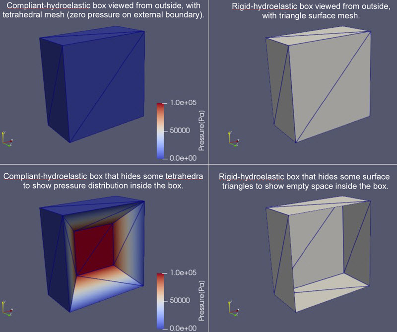
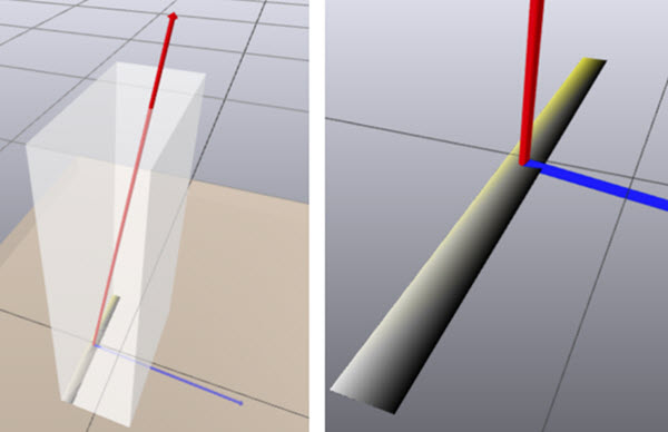
Collision geometries for hydroelastic contact can be either "compliant-hydroelastic" with tetrahedral meshes describing an internal pressure field or "rigid-hydroelastic" with triangle surface meshes that are regarded as infinitely stiff. The figure below shows examples of a compliant hydroelastic box and a rigid hydroelastic box.
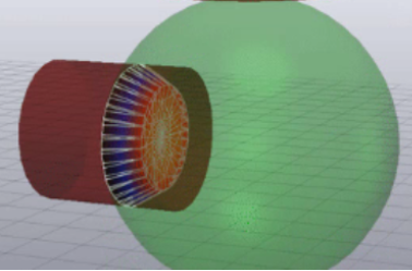
The figure below shows a contact surface between a compliant-hydroelastic cylinder and a compliant-hydroelastic sphere. The contact surface is internal to both solids and is defined as the surface where the two pressure fields are equal.
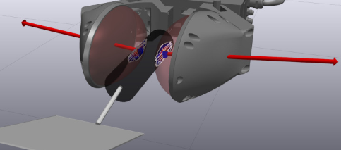
Pictured below, a rigid-hydroelastic cylindrical spatula handle is grasped by two hydroelastic-compliant ellipsoidal bubble grippers. The contact surface between the spatula handle's rigid-hydroelastic geometry and either gripper is on the surface of the rigid-hydroelastic geometry.
Enabling Hydroelastic contact in your simulation
Because MultibodyPlant is responsible for computing the dynamics of the system (and the contact forces are part of that), the ability to enable/disable the hydroelastic contact model is part of MultibodyPlant’s API: drake::multibody::MultibodyPlant::set_contact_model().
There are three different options:
The default model is kHydroelasticWithFallback.
kPoint is the implementation of the point contact model (see Modeling Compliant Contact).
Models kHydroelastic and kHydroelasticWithFallback will both enable the hydroelastic contact. For forces to be created from hydroelastic contact, geometries need to have hydroelastic representations (see Hydroelastic Quick-start, Creating hydroelastic representations of collision geometries).
kHydroelastic is a strict contact model that will attempt to create a hydroelastic contact surface whenever a geometry with a hydroelastic representation appears to be in contact (based on broad-phase bounding volume culling). With this contact model, the simulator will throw an exception if:
- The contact is between two geometries with rigid hydroelastic representation, or
- The contact is between a geometry with a hydroelastic representation and one without.
Collisions between two geometries where neither has a hydroelastic representation are simply ignored.
kHydroelasticWithFallback provides “fallback” behavior for when kHydroelastic would throw. When those scenarios are detected, it uses the point contact model between the colliding geometries so that the contact can be accounted for and produce contact forces. As the implementation evolves, more and more contact will be captured with hydroelastic contact and the circumstances in which the point-contact fallback is applied will decrease.
Creating hydroelastic representations of collision geometries
There are three ways to configure hydroelastic representations for collision geometries:
If none of the above are done, no geometry in drake::geometry::SceneGraph has a hydroelastic representation. So, enabling hydroelastic contact in MultibodyPlant, but forgetting to configure the geometries will lead to either simulation crashes or point contact-based forces.
In order for a mesh to be given a hydroelastic representation, it must be assigned certain properties. The exact properties it needs depends on the Shape type and whether it is rigid or compliant. Some properties can be defined, but if they are absent they’ll be provided by MultibodyPlant. First we’ll discuss each of the properties and then discuss how they can be specified.
Properties for hydroelastic contact
- Hydroelastic classification
- To have a hydroelastic representation, a shape needs to be classified as either “compliant” or “rigid”. This must be explicit – there are no implicit assumptions. Otherwise, it will participate in point contact only.
- Resolution hint (meters)
- A positive real value in meters.
- Most shapes (capsules, cylinders, ellipsoids, spheres) need to be tessellated into meshes. The resolution hint controls the fineness of the meshes.
- For all tessellated geometries, Drake puts hard limits on the effect of the resolution hint property. There is a limit to how fine Drake will tessellate a primitive. Drake has hard-coded internal limits that are still very generous (approximately 100 million tetrahedra or triangles) which should be more than enough for any application. In practice, resolution hints will be quite “large” as coarser meshes are typically more desirable.
- Notes on choosing a value:
- Generally, the coarsest mesh that produces desirable results will allow the simulation to run as efficiently as possible.
- The coarsest mesh will typically be generated when the resolution is equal to the geometry’s maximum measure (see the details below).
- If tessellation artifacts become obvious in the simulation, either make the object more compliant (see hydroelastic modulus) or increase the resolution (as discussed for the various shapes below).
- Geometric detail:
- For each geometry type, the resolution hint works with some (maybe abstract) choice of a representative circle, and its effect is defined in terms of the circumference of that circle. The resolution hint is the target length of each edge of the tessellated mesh around the circle. The circle will have N = ⌈2πr/h⌉ edges, where r is the capsule radius and h is the resolution hint. The number N changes discontinuously as h changes. However, generally, decreasing the resolution hint by some factor will increase the number of edges by that same factor. The number of elements will grow quadratically.
- Sphere
- The representative circle is the great circle of the sphere.
- Cylinder
- The representative circle is the base of the cylinder.
- Capsule
- The representative circle is the base of the cylinder, which is also the great circle of each hemisphere.
- Ellipsoid
- The representative circle is an abstract circle whose radius is that of the largest semi-axis of the elllipsoid.
- Resolution hint has no effect on Box.
- Hydroelastic modulus (Pa (N/m²))
- This is the measure of how stiff the material is. It directly defines how much pressure is exerted given a certain amount of penetration. More pressure leads to greater forces. Larger values create stiffer objects. An infinite modulus is mathematically equivalent to a “rigid” object. (Although, it is definitely better, in that case, to simply declare it “rigid”.)
- Estimation of Hydroelastic Parameters shows how to estimate the hydroelastic modulus using analytical formulas.
- Notes on choosing a value:
- Starting with the value for Young’s modulus is not unreasonable. However, large values (corresponding for instance to the Young’s modulus of metals) can cause numerical problems. In practice, values as high or larger than 10⁸ Pa are seldom used. Refer to Estimation of Hydroelastic Parameters for further details.
- For large modulus values, the resolution of the representations matter more. A very high modulus will keep the contact near the surface of the geometry, exposing tessellation artifacts. A smaller modulus has a smoothing effect.
- This is only required for shapes declared to be “compliant”. It can be defined for shapes declared as “rigid”, but the value will be ignored. (It can be convenient to always define it to enable tests where one might toggle the classification between rigid and compliant such that the compliant declaration is always well formed.)
- Declaring a geometry to be compliant but not providing a valid hydroelastic modulus will produce an error at the time the geometry is added to SceneGraph.
- Hunt-Crossley dissipation (s/m)
- A non-negative real value.
- This gives the contact an energy-damping property.
- The larger the value, the more energy is damped.
- If no value is provided, MultibodyPlant provides a default value of zero.
- Notes on choosing a value:
- For objects that are nominally rigid, starting with zero-damping is good.
- If the behavior seems “jittery”, gradually increase the amount of dissipation. Typical values would remain in the range [0, 100] with 10 to 50 being a typical damping amount.
- The inverse of the Hunt-Crossley dissipation is the maximum bounce velocity between two objects. Therefore, if maximum bounce velocities of 10 cm/s are acceptable, a dissipation of 10 s/m will keep bounce velocities bounded to this range.
- Warning: values larger than about 500 s/m are unphysical and typically lead to numerical problems. Due to time discretization errors, the user will see objects that take a long time to go back to their rest state.
- Remember, as this value increases, your simulation will lose energy at a higher rate.
- See Modeling Dissipation for details.
- Margin (m), see Margin for Hydroelastic Contact
- A non-negative real value.
- Used in discrete mode to mitigate spurious oscillations in the contact of nearly flat surfaces.
- Notes on choosing a value:
- Slab thickness
- A positive real value in meters
- Only used for compliant half spaces. Declaring a half space to be compliant but lacking a value for slab thickness will cause the simulation to error out.
- A measure of the thickness of the compliant material near the boundary of the half space.
- A compliant half space can be made more rigid by:
- Increasing the hydroelastic modulus and fixing slab thickness.
- Fixing the hydroelastic modulus and decreasing the slab thickness.
- Increasing the hydroelastic modulus and decreasing the slab thickness.
Assigning hydroelastic properties to geometries
Properties can be assigned to geometries inside a URDF or SDFormat file using some custom Drake XML tags. Alternatively, the properties can be assigned programmatically.
Assigning hydroelastic properties in file specifications
Drake has introduced a number of custom tags to provide a uniform language to specify hydroelastic properties in both URDF and SDFormat. The tag names are the same but the values are expressed differently (to align with the practices common to URDF and SDFormat). For example, consider a custom tag <drake:foo> that takes a single integer value. In an SDFormat file it would look like:
<drake:foo>17</drake:foo>
But in a URDF file it would look like this:
<drake:foo value=”17”/>
Both URDF and SDFormat files define a <collision> tag. This tag contains the tag for specifying the geometry type and associated properties. The hydroelastic properties can be specified as a child of the <collision> tag. Consider the following SDFormat example:
…
  <collision name="body1_collision">
    <geometry>
      ...
    </geometry>
    <drake:proximity_properties>
      <drake:compliant_hydroelastic/>
      <drake:mesh_resolution_hint>0.1</drake:mesh_resolution_hint>
      <drake:hydroelastic_modulus>5e7</drake:hydroelastic_modulus>
      <drake:hunt_crossley_dissipation>1.25</drake:hunt_crossley_dissipation>
    </drake:proximity_properties>
  </collision>
…
and the following equivalent URDF example:
…
  <collision name="body1_collision">
    <geometry>
      ...
    </geometry>
    <drake:proximity_properties>
      <drake:compliant_hydroelastic/>
      <drake:mesh_resolution_hint value="0.1"/>
      <drake:hydroelastic_modulus value="5e7/>
      <drake:hunt_crossley_dissipation value="1.25/>
    </drake:proximity_properties>
  </collision>
…
For a body, we’ve defined a collision geometry called “body1_collision”. Inside the <collision> tag (as a sibling to the <geometry> tag), we’ve introduced the Drake-specific <drake:proximity_properties> tag. In it we’ve defined the geometry to be compliant for hydroelastic contact and specified its resolution hint, its hydroelastic modulus, and its dissipation.
Let’s look at the specific tags:
- <drake:proximity_properties>: This is the container for all Drake-specific proximity property values.
- The following tags define hydroelastic properties for the collision geometry and would be contained in the <drake:proximity_properties> tag.
- In the name of completeness, the following tags would be children of the <drake:proximity_properties> tag as well, but are not restricted to use with hydroelastic contact.
- <drake:point_contact_stiffness>: Only used when this geometry is for point contact. Defines the compliance of the point contact. This property is allowed to exist even if the geometry has been specified to be of hydroelastic type, it will have no effect on hydroelastic computations.
- <drake:mu_static> The coefficient for static friction; this applies to both point contact and hydroelastic contact.
- <drake:mu_dynamic> The coefficient for dynamic friction; this applies to both point contact and hydroelastic contact.
Assigning hydroelastic properties in code
Hydroelastic properties can be set to objects programmatically via the following APIs (see their documentation for further details):
- AddContactMaterial()
- AddRigidHydroelasticProperties()
- AddCompliantHydroelasticProperties()
- AddCompliantHydroelasticPropertiesForHalfSpace()
Some extra notes:
AddContactMaterial() isn’t hydroelastic contact specific, but does provide a mechanism for setting the friction coefficients that hydroelastic and point contact models both use.
AddRigidHydroelasticProperties() is overloaded. One version accepts a value for resolution hint, one does not. When in doubt which to use, it is harmless to provide a resolution hint value that would be ignored for some geometries, but failing to provide one where necessary will cause the simulation to throw an exception. Note the special case for declaring a compliant half space – it takes the required slab thickness parameter in addition to the hydroelastic modulus value.
Visualizing hydroelastic contact
Start Meldis by:
$ bazel run //tools:meldis -- --open-window &
Run a simulation with hydroelastic contact model; for example,
$ bazel run //examples/hydroelastic/ball_plate:ball_plate_run_dynamics -- \
   --mbp_dt=0.001 --x0=0.10 --z0=0.15 --vz=-7.0 --simulation_time=0.015
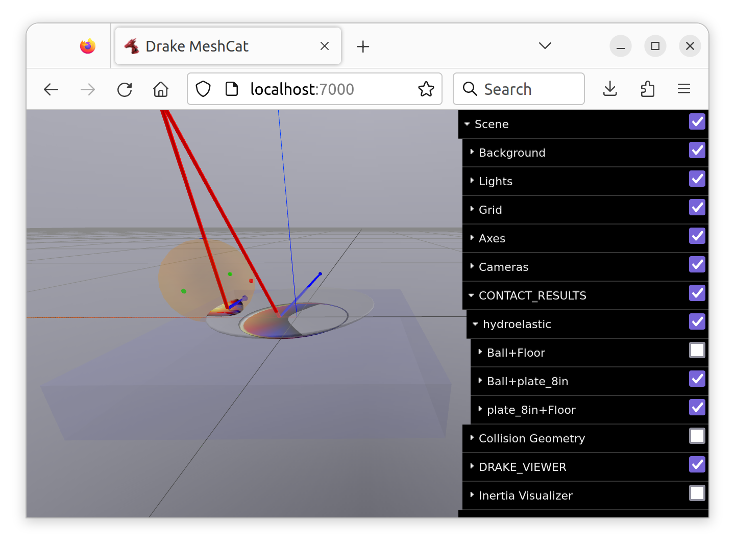
At the time of this writing, the Meldis view of this example looks like this:
In the above picture, we see two red force vectors acting at the centroids of the two contact surfaces and also the two blue moment vectors. One contact surface represents the ball pushing the dinner plate down. The other contact surface represents the rectangular floor pushing the dinner plate up. (Gravity forces are not shown, nor is the contact between the ball and the floor.) Notice that only approximately half of the bottom of the plate makes contact with the floor.
The Scene panel can toggle on/off many different aspects of the visualization using checkboxes, including: which contacts are shown, whether to view the illustration (visual) geometry and/or collision (proximity) geometry and/or the bodies' inertia, as well as sliders for controlling transparency to better view overlapping shapes.
When viewing collisions, note that red arrows indicate a hydroelastic contact, with an associated contact patch. Green arrows indicate point contact, which does not have any contact patch.
Pitfalls/Troubleshooting
Here are various ways that hydroelastic contact may surprise you.
- A rigid body is not a rigid hydroelastic body until users say so (see Creating hydroelastic representations of collision geometries). Otherwise, it is ignored by the hydroelastic contact model and might get point contact instead.
- Users need to call AddRigidHydroelasticProperties() or use the URDF or SDFormat tag <drake:rigid_hydroelastic/>.
- Backface culling – the visualized contact surface is not what you expect. Or, “Why are there holes?”
- Hydroelastic modulus is not properly a material property; it combines material and geometry.
- Make the sphere bigger, the force gets weaker for the same contact surface.
- “I don’t seem to be getting any contact surfaces although my spheres are clearly overlapping!” Depending on how coarsely you tessellated your geometry (a sphere, at its coarsest, is an octahedron), there can be a large amount of error between the primitive surface and discrete mesh’s surface. Make sure you visualize the hydro meshes and have what you expect.
- Stiff and coarse is seldom a good thing. The stiffer an object is, the more the details of the discrete tessellation will directly contribute to the dynamics.
- Getting moments out of the contact depends on how many elements are in the contact surface. If the elements of the two contributing meshes are much larger than the actual contact surface, the contact can become, in essence, point contact.
- Half spaces are not represented by meshes. They don’t contribute any geometry to the resultant contact surface. The contact surface’s refinement will depend on the other geometry’s level of refinement.
Tips and Tricks
This is a random collection of things we can do to maximize the benefits of the hydroelastic contact model. Some of these tricks accommodate current implementation limitations, and some are to work within the theoretical framework.
Gaming the model
- Rigid meshes need not be closed. You can use this to provide fine grained control over where a contact surface can actually exist. Be careful to have a consistent direction of surface normals on the triangles. They should point outward.
- For a given relative configuration between bodies, the magnitude of force can be tuned in two ways: increasing the hydroelastic modulus and/or scaling the geometry up (in essence, increasing the average penetration depth).
Appendix A: Current state of implementation
This section will be updated as the scope and feature set of hydroelastic contact is advanced. The main crux of this section is to clearly indicate what can and cannot be done with hydroelastic contact.
What can you do with hydroelastic contact?
- Hydroelastic contact can be used with MultibodyPlant in either continuous or discrete mode.
- You can visualize the contact surfaces, their pressure fields, and the resultant contact forces in MeshCat as the simulation progresses. However, for playing back recordings in MeshCat, only the contact forces and moments are available (see issue 19142).
- All Drake Shape types can be used to create rigid hydroelastic bodies (this includes arbitrary meshes defined as OBJs).
- Drake primitive Shape types (Box, Capsule, Cylinder, Ellipsoid, HalfSpace, and Cylinder) can all be used to create both compliant hydroelastic bodies and rigid hydroelastic bodies.
- The Drake Convex Shape type can be used both as a compliant hydroelastic body and a rigid hydroelastic body. To use Convex, add the custom tag <drake:declare_convex/> tag under the <mesh> tag in either an SDFormat or URDF file.
- The Drake Mesh Shape type can be used as a compliant hydroelastic body using a tetrahedral mesh in VTK file. See examples/hydroelastic/python_nonconvex_mesh.
What can’t you do with hydroelastic contact?
- You can’t get contact surfaces between two rigid hydroelastic geometries. The contact surface between rigid geometries is ill defined and will most likely never be supported. The default drake::multibody::ContactModel::kHydroelasticWithFallback uses compliant point contact as a reliable default. See Enabling Hydroelastic contact in your simulation.
- Hydroelastics cannot model true deformations given the model does not introduce state. Therefore effects such as tangential compliance or short time scale waves are not captured by the model. Currently we are actively developing code for deformable bodies in DeformableModel.
Current dissipation models
- The TAMSI (DiscreteContactApproximation::kTamsi), Similar (DiscreteContactApproximation::kSimilar), and Lagged (DiscreteContactApproximation::kLagged) model approximations use a Hunt-Crossley model of dissipation, parameterized by hunt_crossley_dissipation, for both point and hydroelastic contact. The SAP approximation parameter relaxation_time is ignored by these approximations.
- The SAP model approximation (DiscreteContactApproximation::kSap) uses a linear Kelvin–Voigt model of dissipation parameterized by relaxation_time, for both point and hydroelastic contact. The Hunt-Crossley dissipation parameter is ignored by this approximation.
- We allow the user to specify both hunt_crossley_dissipation (TAMSI, Similar and Lagged discrete approximations as well as continuous plant model) and relaxation_time (SAP approximation specific parameter) on the model, but the parameter may be ignored depending on your plant configuration. See the documentation for that in the MultibodyPlant documentation.
Appendix B: Examples and Tutorials
Sources referenced within this documentation
- [Elandt 2019] Elandt, R., Drumwright, E., Sherman, M., & Ruina, A. (2019, November). A pressure field model for fast, robust approximation of net contact force and moment between nominally rigid objects. In 2019 IEEE/RSJ International Conference on Intelligent Robots and Systems(IROS) (pp. 8238-8245). IEEE. https://arxiv.org/abs/1904.11433 .
- [Masterjohn 2022] Masterjohn, J., Guoy, D., Shepherd, J., & Castro, A. (2022). Velocity Level Approximation of Pressure Field Contact Patches. In 2022 IEEE/RSJ International Conference on Intelligent Robots and Systems(IROS). https://arxiv.org/abs/2110.04157 .
- [Sherman 2022] Sherman, M. (2022, June). Rethinking Contact Simulation for Robot Manipulation. Blog post in Medium. https://medium.com/toyotaresearch/rethinking-contact-simulation-for-robot-manipulation-434a56b5ec88 .