
For instructions on how to run these tutorial notebooks, please see the index.
If you are not familiar with Drake, see the index or study authoring_multibody_simulation.ipynb. You can also find more information in Hydroelastic Contact User Guide here.
This tutorial shows you how to set up dynamic simulations with hydroelastic contacts. It also shows you how to report contact results numerically and visualize them in MeshCat. For context, we use a simple example of a compliant block dropped onto a rigid horizontal rectangular plate. Contact forces are calculated and visualized.
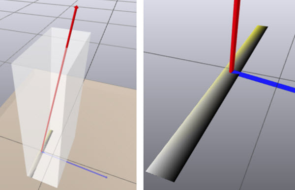
For example, the below-left picture shows one frame of the block's contact, with the complex set of contact forces visualized as a contact wrench (force/torque), with the force as a red arrow and the torque as a blue arrow. The below-right picture zooms into the hydroelastic contact surface showing pressure distribution, with black for zero pressure (right edge) and white for highest pressure (left-edge). Because the block is rocking back and forth on the plate, the contact patch is located at one edge of the bottom face of the block instead of the entire rectangular face.
Drake's Hydroelastic Contact Model evolved at Toyota Research Institute in conjunction with the work by Ryan Elandt who invented the Pressure Field Contact (PFC) model. Ryan's PhD thesis describes the usefulness of the PFC model:
"...This model is useful in situations where deformation in the contact region is qualitatively important, but need not be accurate. PFC is a model of, and not a convergent approximation of, continuum mechanics. In PFC, each of the two contacting objects is assigned an immutable internal virtual pressure field. ... the PFC contact surface is defined as the set of points where the two pressure fields are equal. ..."
For an excellent overview of hydroelastic contact, read these two articles (less than 10 minutes each):
Generally, hydroelastic contact is faster than Finite Element Analysis (FEA) and more continuous and stable than point contact models, particularly in realistic situations involving friction, rolling, energy dissipation, and non-convex geometries. Hydroelastic contact does not include deformation (as in FEA) and is slower than the point contact models used in some simulators (including an optional one in Drake).
When two rigid bodies are interacting due to hydroelastic contact, neither has actual mechanical deformation, i.e., the bodys' mass, center of mass, and inertia properties are unaffected by hydroelastic contact. However, their force interaction is calculated as if there were deformation.
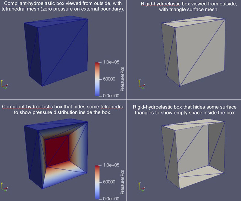
There are two types of hydroelastic geometries. The first, called "compliant-hydroelastic", is a solid which contains a tetrahedral mesh that describes an internal pressure field. (Note: the pressure on the solid's surface is zero, and for fast computation, the simulator pre-calculates the internal pressure field -- before a contact is possible). The second, called "rigid-hydroelastic", only has a triangle surface mesh (hence the geometry may be a solid or a surface) and is regarded as infinitely stiff.
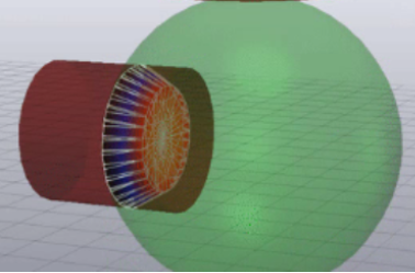
The figure below shows contact between a compliant-hydroelastic cylinder and a compliant-hydroelastic sphere. The contact surface is internal to both solids and is defined as the surface where the two pressure fields are equal. The shading on the contact surface shows pressure distribution varying from black (zero pressure) to red (high pressure). Mathematically, the contact surface is a blending surface between the intersecting portions of the cylinder's surface and the sphere's surface. Conceptually, for two similarly-sized spheres, the contact surface is closer to the surface of the sphere that has the larger hydroelastic modulus. See this section in Drake's discussion of compliant contact.
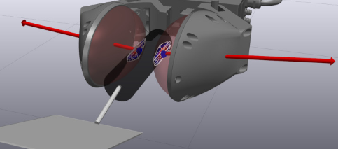
Since a rigid-hydroelastic geometry is regarded as infinitely stiff, the contact surface between a compliant-hydroelastic geometry and a rigid-hydroelastic geometry is on the surface of the rigid-hydroelastic geometry. As pictured below, two hydroelastic-compliant ellipsoidal bubble fingers are in contact with a rigid-hydroelastic cylindrical spatula handle. Hence, the contact surfaces are on the surface of the spatula handle.
In general, consider using compliant-hydroelastic geometries because the object's stiffness can be specified through its hydroelastic modulus to be as compliant as rubber or as stiff as steel. Compliant-hydroelastic geometries need tetrahedral meshes. Drake can automatically generate tetrahedral meshes of compliant-hydroelastic geometries for built-in shapes such as spheres, ellipsoids, cylinders, capsules, boxes, and for solids with a convex surface mesh. For non-convex objects, each mesh must be provided as a VTK file (not a .obj file) containing a tetrahedral mesh to use them as compliant-hydroelastic geometries.
Compliant-hydroelastic objects interact well with either compliant-hydroelastic objects or with rigid-hydroelastic objects.
Alternatively, an important use for rigid-hydroelastic geometry is for an object with a non-convex surface mesh (e.g., .obj file) whose associated tetrahedral volume mesh is not readily available. Currently, a rigid-hydroelastic geometry can only interact with compliant-hydroelastic objects. If it interacts with another rigid-hydroelastic object, the simulator reverts to point contact. The table below elaborates these and other cases.
| rigid-hydroelastic geometry | compliant-hydroelastic geometry | |
|---|---|---|
| rigid-hydroelastic geometry | point contact | hydroelastic contact |
| compliant-hydroelastic geometry | hydroelastic contact | hydroelastic contact |
| non-hydroelastic geometry | point contact | point contact |
This tutorial shows you how to:
Define SDFormat string for a compliant-hydroelastic box.
Define SDFormat string for a rigid-hydroelastic box.
Create Diagram of MultibodyPlant using the two boxes.
Visualize the simulation.
Create a LeafSystem to numerically report contact results at the end of a simulation.
Add ContactVisualizer to visualize contact results.
See the section Viewing models in the tutorial Authoring a Multibody Simulation for an introduction to MeshCat.
from pydrake.geometry import StartMeshcat

# Start the visualizer. The cell will output an HTTP link after the execution.
# Click the link and a MeshCat tab should appear in your browser.
meshcat = StartMeshcat()
INFO:drake:Meshcat listening for connections at http://localhost:7000
Make sure you have the MeshCat tab opened in your browser; the link is shown immediately above.
We will create and visualize a compliant-hydroelastic box with SDFormat string.
We will use ModelVisualizer to verify the SDFormat description.
It will tell MeshCat to show the box.
First we create a visual geometry of a box of size 10cm x 20cm x 40cm. Observe in MeshCat the X(red), Y(green), and Z(blue) axes. The <size>0.10 0.20 0.40</size> specifies the dimensions of the box in meters. The <diffuse> tag specifies the RGB and alpha values between 0 and 1.
from pydrake.visualization import ModelVisualizer

visual_box_sdf = """<?xml version="1.0"?>
<sdf version="1.7">
  <model name="CompliantBox">
    <pose>0 0 0 0 0 0</pose>
    <link name="compliant_box">
      <visual name="visual">
        <geometry>
          <box>
            <size>0.10 0.20 0.40</size>
          </box>
        </geometry>
        <material>
          <diffuse>1.0 1.0 1.0 0.5</diffuse>
        </material>
      </visual>
    </link>
  </model>
</sdf>
"""

# Visualize the SDFormat string you just defined.
visualizer = ModelVisualizer(meshcat=meshcat, visualize_frames=True)
visualizer.parser().AddModelsFromString(visual_box_sdf, "sdf")
visualizer.Run(loop_once=True)
We will add the <collision> block with hydroelastic properties. Without <collision>, our object cannot make contact in the simulation.
We specify the same collision geometry (box of size 10x20x40 centimeters) as the visual geometry.
Drake also uses the term proximity for collision. This is the <drake:proximity_properties> block that control hydroelastic contacts:
    <drake:proximity_properties>
      <drake:compliant_hydroelastic/>
      <drake:hydroelastic_modulus>1e7</drake:hydroelastic_modulus>
      <drake:mu_dynamic>0.5</drake:mu_dynamic>
      <drake:hunt_crossley_dissipation>1.25</drake:hunt_crossley_dissipation>
    </drake:proximity_properties>
Use <drake:compliant_hydroelastic/> to specify a compliant-hydroelastic object.
We set <drake:hydroelastic_modulus> to 1e7 Pascals. It is comparable to high-density polyethylene (HDPE) with 1 GPa Young's modulus. Hydroelastic modulus is not a physical property but rather a numerical parameter to tune our contact model. As a rule of thumb, set hydroelastic modulus to about 1/100 of Young's modulus.
We set <drake:mu_dynamic> (unitless) to 0.5 for the coefficient of dynamic (i.e., kinetic) friction.
We set <drake:hunt_crossley_dissipation> to 1.25 seconds/meter as the dissipation constant for the Hunt & Crossley model.
from pydrake.visualization import ModelVisualizer

collision_box_sdf = """<?xml version="1.0"?>
<sdf version="1.7">
  <model name="CompliantBox">
    <pose>0 0 0 0 0 0</pose>
    <link name="compliant_box">
      <collision name="collision">
        <geometry>
          <box>
            <size>0.10 0.20 0.40</size>
          </box>
        </geometry>
        <drake:proximity_properties>
          <drake:compliant_hydroelastic/>
          <drake:hydroelastic_modulus>1e7</drake:hydroelastic_modulus>
          <drake:mu_dynamic>0.5</drake:mu_dynamic>
          <drake:hunt_crossley_dissipation>1.25</drake:hunt_crossley_dissipation>
        </drake:proximity_properties>
      </collision>
      <visual name="visual">
        <geometry>
          <box>
            <size>0.10 0.20 0.40</size>
          </box>
        </geometry>
        <material>
          <diffuse>1.0 1.0 1.0 0.5</diffuse>
        </material>
      </visual>
    </link>
  </model>
</sdf>
"""

# Visualize the SDFormat string you just defined.
visualizer = ModelVisualizer(meshcat=meshcat, visualize_frames=True)
visualizer.parser().AddModelsFromString(collision_box_sdf, "sdf")
visualizer.Run(loop_once=True)
In order to simulate dynamics, we will add <mass> of 1kg and <inertia> matrix.
The <inertia> of the box about its center of mass is calculated with:
Ixx = m(s.y² + s.z²)/12
Iyy = m(s.x² + s.z²)/12
Izz = m(s.x² + s.y²)/12
where s.x, s.y, and s.z are the dimensions of the box.
In practice, we can use SpatialInertia.SolidBoxWithMass() as shown below and copy the numbers into SDFormat string afterwards. See documentation of SpatialInertia for description of the 6x6 matrix.
from pydrake.multibody.tree import SpatialInertia

spatial_inertia = SpatialInertia.SolidBoxWithMass(
          mass=1, lx=0.1, ly=0.2, lz=0.4)
mass = spatial_inertia.get_mass()
center_of_mass = spatial_inertia.get_com()
matrix6 = spatial_inertia.CopyToFullMatrix6()

print(f"mass = {mass}\n")
print(f"p_PScm = center of mass = {center_of_mass}\n")
print(f"I_SP = rotational inertia = \n{matrix6[:3, :3]}\n")
mass = 1.0

p_PScm = center of mass = [0. 0. 0.]

I_SP = rotational inertia =
[[0.01666667 0.         0.        ]
 [0.         0.01416667 0.        ]
 [0.         0.         0.00416667]]
The function compliant_box() below returns SDFormat description of the compliant-hydroelastic box given hydroelastic_modulus. We will use this function later when we experiment with different values of hydroelastic modulus. The numbers in <inertial> block are copied from the result of exercising the above code with SpatialInertia.
Notice that the parameter hydroelastic_modulus is a character string '1e7' (it is enclosed by single quote '), not a floating-point number 1e7, so that the SDFormat description does not lose precision due to formatting.
from pydrake.visualization import ModelVisualizer

# Define a compliant-hydroelastic box from
# a given hydroelastic modulus.
def compliant_box(hydroelastic_modulus='1e7'):
    return f"""<?xml version="1.0"?>
    <sdf version="1.7">
      <model name="CompliantBox">
        <pose>0 0 0 0 0 0</pose>
        <link name="compliant_box">
          <inertial>
            <mass>1.0</mass>
            <inertia>
              <ixx>0.016666</ixx> <ixy>0.0</ixy> <ixz>0.0</ixz>
              <iyy>0.014166</iyy> <iyz>0.0</iyz>
              <izz>0.004166</izz>
            </inertia>
          </inertial>
          <collision name="collision">
            <geometry>
              <box>
                <size>0.10 0.20 0.40</size>
              </box>
            </geometry>
            <drake:proximity_properties>
              <drake:compliant_hydroelastic/>
              <drake:hydroelastic_modulus>{hydroelastic_modulus}</drake:hydroelastic_modulus>
              <drake:mu_dynamic>0.5</drake:mu_dynamic>
              <drake:hunt_crossley_dissipation>1.25</drake:hunt_crossley_dissipation>
            </drake:proximity_properties>
          </collision>
          <visual name="visual">
            <geometry>
              <box>
                <size>0.10 0.20 0.40</size>
              </box>
            </geometry>
            <material>
              <diffuse>1.0 1.0 1.0 0.5</diffuse>
            </material>
          </visual>
        </link>
      </model>
    </sdf>
    """

compliant_box_sdf = compliant_box()
print(compliant_box_sdf)

# Visualize the SDFormat string you just defined.
visualizer = ModelVisualizer(meshcat=meshcat, visualize_frames=True)
visualizer.parser().AddModelsFromString(compliant_box_sdf, "sdf")
visualizer.Run(loop_once=True)
<?xml version="1.0"?>
    <sdf version="1.7">
      <model name="CompliantBox">
        <pose>0 0 0 0 0 0</pose>
        <link name="compliant_box">
          <inertial>
            <mass>1.0</mass>
            <inertia>
              <ixx>0.016666</ixx> <ixy>0.0</ixy> <ixz>0.0</ixz>
              <iyy>0.014166</iyy> <iyz>0.0</iyz>
              <izz>0.004166</izz>
            </inertia>
          </inertial>
          <collision name="collision">
            <geometry>
              <box>
                <size>0.10 0.20 0.40</size>
              </box>
            </geometry>
            <drake:proximity_properties>
              <drake:compliant_hydroelastic/>
              <drake:hydroelastic_modulus>1e7</drake:hydroelastic_modulus>
              <drake:mu_dynamic>0.5</drake:mu_dynamic>
              <drake:hunt_crossley_dissipation>1.25</drake:hunt_crossley_dissipation>
            </drake:proximity_properties>
          </collision>
          <visual name="visual">
            <geometry>
              <box>
                <size>0.10 0.20 0.40</size>
              </box>
            </geometry>
            <material>
              <diffuse>1.0 1.0 1.0 0.5</diffuse>
            </material>
          </visual>
        </link>
      </model>
    </sdf>
The following SDFormat string specifies a rigid-hydroelastic box. It is similar to the compliant-hydroelastic box.
Both the <visual> and <collision> geometries are boxes of size 60cm x 1m x 5cm. Observe in MeshCat the X(red), Y(green), and Z(blue) axes.
Use the tag <drake:rigid_hydroelastic/> to specify a rigid-hydroelastic geometry. It does not use <drake:hydroelastic_modulus>. Intuitively it has infinite hydroelastic modulus.
This rigid-hydroelastic box uses the same friction coefficient and dissipation constants as the previous compliant-hydroelastic box.
We do not specify <mass> and <inertia> of the rigid box because, in the next section when we set up Diagram, we will fix the rigid box to the world frame. It will not move.
The <frame name="top_surface"> is a frame at the top of the box with the tag:
<pose relative_to="rigid_box_link">0 0 0.025 0 0 0</pose>
It is at 2.5cm (half of the box's height) above the center of the box. In the next section, we will create a scene that places the top_surface frame at the world's origin.
from pydrake.visualization import ModelVisualizer

# Create a rigid-hydroelastic table top
rigid_box_sdf = """<?xml version="1.0"?>
<sdf version="1.7">
  <model name="RigidBox">
    <link name="rigid_box_link">
      <visual name="visual">
        <pose>0 0 0 0 0 0</pose>
        <geometry>
          <box>
            <size>0.6 1.0 0.05</size>
          </box>
        </geometry>
        <material>
         <diffuse>0.9 0.8 0.7 0.5</diffuse>
        </material>
      </visual>
      <collision name="collision">
        <pose>0 0 0 0 0 0</pose>
        <geometry>
          <box>
            <size>0.6 1.0 0.05</size>
          </box>
        </geometry>
        <drake:proximity_properties>
          <drake:rigid_hydroelastic/>
          <drake:mu_dynamic>0.5</drake:mu_dynamic>
          <drake:hunt_crossley_dissipation>1.25</drake:hunt_crossley_dissipation>
        </drake:proximity_properties>
      </collision>
    </link>
    <frame name="top_surface">
      <pose relative_to="rigid_box_link">0 0 0.025 0 0 0</pose>
    </frame>
  </model>
</sdf>
"""

# Visualize the SDFormat string you just defined.
visualizer = ModelVisualizer(meshcat=meshcat, visualize_frames=True)
visualizer.parser().AddModelsFromString(rigid_box_sdf, "sdf")
visualizer.Run(loop_once=True)
The function add_scene() below creates a scene using the two boxes that we created.
It uses DiagramBuilder to create MultibodyPlant and SceneGraph. It uses Parser to add the two SDFormat strings of the two boxes into Diagram of the scene.
It sets discrete_contact_approximation to "similar" for stability during high impacts. See DiscreteContactApproximation.
It fixes the rigid box's top surface to the world frame by calling WeldFrames().
It places the compliant box 1 meter above the rigid box.
After this step, the next section will add visualization to DiagramBuilder.
from pydrake.math import RigidTransform
from pydrake.multibody.parsing import Parser
from pydrake.multibody.plant import AddMultibodyPlant, MultibodyPlantConfig
from pydrake.systems.framework import DiagramBuilder

def clear_meshcat():
    # Clear MeshCat window from the previous blocks.
    meshcat.Delete()
    meshcat.DeleteAddedControls()

def add_scene(time_step=1e-3):
    builder = DiagramBuilder()
    plant, scene_graph = AddMultibodyPlant(
        MultibodyPlantConfig(
            time_step=time_step,
            discrete_contact_approximation="similar"),
        builder)
    parser = Parser(builder)

    # Load the table top and the box we created.
    parser.AddModelsFromString(compliant_box_sdf, "sdf")
    parser.AddModelsFromString(rigid_box_sdf, "sdf")

    # Weld the rigid box to the world so that it's fixed during simulation.
    # The top surface passes the world's origin.
    plant.WeldFrames(plant.world_frame(),
                     plant.GetFrameByName("top_surface"))

    # Finalize the plant after loading the scene.
    plant.Finalize()

    # Set how high the center of the compliant box is from the world's origin.
    # W = the world's frame
    # C = frame at the center of the compliant box
    X_WC = RigidTransform(p=[0, 0, 1])
    plant.SetDefaultFloatingBaseBodyPose(plant.GetBodyByName("compliant_box"), X_WC)

    return builder, plant
The function add_scene() above does not have visualization, so we will do it in the function add_viz() below.
It uses DiagramBuilder from add_scene(). The meshcat interface represents the same MeshCat window that we have been using.
We set the publish_period to 1/256 to publish 256 frames per simulated second. In this example, we publish frequently so we can better see changes in contact. See documentation of VisualizationConfig for more details.
At this step we set publish_contacts to False, we will set up contact visualization near the end of this tutorial.
We test the creation of Diagram by simulating for 0 second. It shows the compliant box 1 meter above the rigid box. You might have to zoom out to see both boxes at the same time.
from pydrake.visualization import ApplyVisualizationConfig, VisualizationConfig

def add_viz(builder, plant):
    ApplyVisualizationConfig(
        config=VisualizationConfig(
                   publish_period = 1 / 256.0,
                   publish_contacts = False),
        builder=builder, meshcat=meshcat)

    return builder, plant


from pydrake.systems.analysis import Simulator

# Test creation of the diagram by simulating for 0 second.
# For now, use only the DiagramBuilder from the first return value and
# ignore the other return value. We will use it later.
clear_meshcat()
builder, plant = add_scene()
add_viz(builder, plant)
simulator = Simulator(builder.Build())
simulator.AdvanceTo(0)
<pydrake.systems.analysis.SimulatorStatus at 0x7ab47f799cb0>
We define the function run_simulation() below. It builds Diagram using DiagramBuilder from the previous step. It passes Diagram to Simulator. It also records simulation result into meshcat for playback later. You should see the compliant box drops down to make contact with the rigid box.
from pydrake.systems.analysis import Simulator

def run_simulation(sim_time, time_step=1e-3):
    clear_meshcat()

    builder, plant = add_scene(time_step)
    add_viz(builder, plant)

    diagram = builder.Build()

    simulator = Simulator(diagram)
    simulator.set_target_realtime_rate(1.)

    meshcat.StartRecording(frames_per_second=256.0)
    simulator.AdvanceTo(sim_time)
    meshcat.StopRecording()


run_simulation(sim_time=6)
The following command meshcat.PublishRecording() will create a playback in the MeshCat tab. It will enable Animations panel in MeshCat tab.
meshcat.PublishRecording()
In the MeshCat window, click on Open Controls if you haven't done it. You should see Animations panel.
Use the play button to replay the animation.
Adjust timeScale to control animation speed. Set it to 0.1 for slower playback to better see changes in contact.
Use pause to stop animation in the middle, and use reset to move the animation back to time 0.
During the playback, you should see the compliant box drops down to make contact with the rigid box and bounces back at about 0.4s simulated time. The gravity will pull it down to make contact again. It will rock back and forth for a few seconds and reach steady state after about 6 seconds simulated time.
You can type time in the Animations panel to go to a particular snapshot in the animation.
One advantage of playback is that you can watch animation at real-time rate with timeScale=1 regardless of how fast or how slow the simulation is. The wall-clock time of the simulation has no consequence to the simulated time that we see in the playback.
We will show you how to report contact results. We will create a simple system to read contact results from MultibodyPlant and print them at the end of simulation.
If you are not familiar with creating a leaf system, please see the tutorial Authoring Leaf Systems.
We will define a leaf system called ContactReporter below. It has an input port that takes ContactResults. When there is a forced publish event, it will print the contact results from its input port. See Publish(self, context) in the code below.
Contact results are available from an output port of MultibodyPlant by calling get_contact_results_output_port(). See documentation of MultibodyPlant's input and output ports for the list of available ports. In the function add_contact_report() below, first we add ContactReporter to the diagram builder from the previous section. Then, we connect the contact results output port of MultibodyPlant to the input port of our ContactReporter.
The simulation in our example has only one contact patch between two geometries, but the code below can report all contact patches from all pairs of geometries from hydroelastics. However, it does not report point_pair_contact_info() in ContactResults.
See documentation of ContactResults, HydroelasticContactInfo, and ContactSurface for more details.
In __init__() of ContactReporter, we declare forced publish event, so it will report contacts only when users call ForcedPublish() (see run_simulation_with_contact_report() in the next section). You can also declare periodic publish events to report contact at the frequency that you specify. See Declare periodic events in documentation of LeafSystem.
from pydrake.common.value import Value
from pydrake.multibody.plant import ContactResults
from pydrake.systems.framework import LeafSystem

class ContactReporter(LeafSystem):
    def __init__(self):
        super().__init__()  # Don't forget to initialize the base class.
        self.DeclareAbstractInputPort(
            name="contact_results",
            model_value=Value(
                # Input port will take ContactResults from MultibodyPlant
                ContactResults()))
        # Calling `ForcedPublish()` will trigger the callback.
        self.DeclareForcedPublishEvent(self.Publish)

    def Publish(self, context):
        print()
        print(f"ContactReporter::Publish() called at time={context.get_time()}")
        contact_results = self.get_input_port().Eval(context)

        num_hydroelastic_contacts = contact_results.num_hydroelastic_contacts()
        print(f"num_hydroelastic_contacts() = {num_hydroelastic_contacts}")

        for c in range(num_hydroelastic_contacts):
            print()
            print(f"hydroelastic_contact_info({c}): {c}-th hydroelastic contact patch")
            hydroelastic_contact_info = contact_results.hydroelastic_contact_info(c)

            spatial_force = hydroelastic_contact_info.F_Ac_W()
            print("F_Ac_W(): spatial force (on body A, at centroid of contact surface, in World frame) = ")
            print(f"{spatial_force}")

            print("contact_surface()")
            contact_surface = hydroelastic_contact_info.contact_surface()
            num_faces = contact_surface.num_faces()
            total_area = contact_surface.total_area()
            centroid = contact_surface.centroid()
            print(f"total_area(): area of contact surface in m^2 = {total_area}")
            print(f"num_faces(): number of polygons or triangles = {num_faces}")
            print(f"centroid(): centroid (in World frame) = {centroid}")

        print()

def add_contact_report(builder, plant):
    contact_reporter = builder.AddSystem(ContactReporter())
    builder.Connect(plant.get_contact_results_output_port(),
                    contact_reporter.get_input_port(0))

    return builder, plant
As shown below, the function run_simulation_with_contact_report() calls ForcedPublish() after the simulation has finished.
The end of the code block calls run_simulation_with_contact_report() with sim_time=0. At time 0, the compliant box starts far above the rigid box. The printout will simply say there is no contact yet. It should look like this:
ContactReporter::Publish() called at time=0.0
num_hydroelastic_contacts() = 0from pydrake.systems.analysis import Simulator
def run_simulation_with_contact_report(sim_time, time_step=1e-3):
clear_meshcat()
builder, plant = add_scene(time_step)
add_viz(builder, plant)
add_contact_report(builder, plant)
diagram = builder.Build()
simulator = Simulator(diagram)
simulator.set_target_realtime_rate(1.)
meshcat.StartRecording(frames_per_second=256.0)
simulator.AdvanceTo(sim_time)
meshcat.StopRecording()
# Forced publish after the simulation has finished.
diagram.ForcedPublish(simulator.get_context())
run_simulation_with_contact_report(sim_time=0)
meshcat.PublishRecording()
ContactReporter::Publish() called at time=0.0
num_hydroelastic_contacts() = 0
We will run it again for 1 second simulated time. Since we will call meshcat.PublishRecording() on the second line, it will look like we drop the compliant box twice. The first animation is directly from the simulation, and the repeated animation is from the playback. You can zoom-in and slow down the playback in MeshCat tab (set timeScale to 0.1) to carefully observe dynamics.
After running the code below, you should see the spatial force F_Ac_W consisting of the torque tau and the force f. The force f is around [-1.52, 0.89, 9.39], expressed in World frame, has the Z component about 9.39 newtons. It is less than 9.81 newtons, which is the gravity force acting on the compliant box with mass 1kg. This is because the compliant box is still rocking back and forth at the 1-second simulated time.
The contact results are reported in World frame.
run_simulation_with_contact_report(sim_time=1)
meshcat.PublishRecording()
ContactReporter::Publish() called at time=1.0
num_hydroelastic_contacts() = 1

hydroelastic_contact_info(0): 0-th hydroelastic contact patch
F_Ac_W(): spatial force (on body A, at centroid of contact surface, in World frame) =
SpatialForce(
  tau=[-0.6287361082654935, -0.05711343608112074, -0.016942635819783385],
  f=[-0.8803968743268051, 3.2001990115006227, 19.556692720092556],
)
contact_surface()
total_area(): area of contact surface in m^2 = 0.015326390259632231
num_faces(): number of polygons or triangles = 36
centroid(): centroid (in World frame) = [ 9.27019418e-03 -1.43371740e-02  1.11022302e-16]
In the next code block, you will run the simulation for 6 seconds to steady state, and you should see f.Z() around 9.81 newtons equal to the gravity force:
f=[-3.35e-05, -4.04e-06, 9.81]
run_simulation_with_contact_report(sim_time=6)
meshcat.PublishRecording()
ContactReporter::Publish() called at time=6.0
num_hydroelastic_contacts() = 1

hydroelastic_contact_info(0): 0-th hydroelastic contact patch
F_Ac_W(): spatial force (on body A, at centroid of contact surface, in World frame) =
SpatialForce(
  tau=[4.908231312633626e-06, 6.713760710781851e-06, 1.2279500656154537e-13],
  f=[2.4790371589329285e-05, -1.7359194516112135e-05, 9.809999999830474],
)
contact_surface()
total_area(): area of contact surface in m^2 = 0.019999999999999997
num_faces(): number of polygons or triangles = 42
centroid(): centroid (in World frame) = [2.13672740e-06 1.23592439e-06 0.00000000e+00]
To visualize contact results, we will add ContactVisualizer to Diagram of the previous section.
The following function add_contact_viz() adds ContactVisualizer to DiagramBuilder using MultibodyPlant and Meshcat.
With newtons_per_meter= 2e1, it will draw a red arrow of length 1 meter for each force of 20 newtons. With newtons_meters_per_meter= 1e-1, it will draw a blue arrow of length 1 meter for each torque of 0.1 newton*meters. The next section will run the simulation.
from pydrake.multibody.meshcat import ContactVisualizer, ContactVisualizerParams


def add_contact_viz(builder, plant):
    contact_viz = ContactVisualizer.AddToBuilder(
        builder, plant, meshcat,
        ContactVisualizerParams(
            publish_period= 1.0 / 256.0,
            newtons_per_meter= 2e1,
            newton_meters_per_meter= 1e-1))

    return builder, plant
The following code will run the simulation. In MeshCat, the red arrow represents the force f, and the blue arrow represents the torque tau. You should see the contact patch moving around together with the force and torque vectors. At the end of simulation, it will also report contact result numerically.
Notice that the code below does not publish the recording yet. The next section will publish the recording for playback.
from pydrake.systems.analysis import Simulator

def run_simulation_with_contact_report_and_viz(sim_time, time_step=1e-3):
    clear_meshcat()

    builder, plant = add_scene(time_step)
    add_viz(builder, plant)
    add_contact_report(builder, plant)
    add_contact_viz(builder, plant)

    diagram = builder.Build()

    simulator = Simulator(diagram)
    simulator.set_target_realtime_rate(1.0)

    meshcat.StartRecording(frames_per_second=256.0)
    simulator.AdvanceTo(sim_time)
    meshcat.StopRecording()

    # Numerically report contact results at the end of simulation.
    diagram.ForcedPublish(simulator.get_context())


run_simulation_with_contact_report_and_viz(sim_time=6)
ContactReporter::Publish() called at time=6.0
num_hydroelastic_contacts() = 1

hydroelastic_contact_info(0): 0-th hydroelastic contact patch
F_Ac_W(): spatial force (on body A, at centroid of contact surface, in World frame) =
SpatialForce(
  tau=[4.908231312633626e-06, 6.713760710781851e-06, 1.2279500656154537e-13],
  f=[2.4790371589329285e-05, -1.7359194516112135e-05, 9.809999999830474],
)
contact_surface()
total_area(): area of contact surface in m^2 = 0.019999999999999997
num_faces(): number of polygons or triangles = 42
centroid(): centroid (in World frame) = [2.13672740e-06 1.23592439e-06 0.00000000e+00]
After running the code below, playback with timeScale = 0.1 or 0.01 to appreciate the contact dynamics. You should see the force and torque vectors oscillate synchronously with the rocking compliant box.
Currently playing back the simulation will show contact force and moment; however, it does not show contact patch appropriately, which could be confusing. The code below deletes the contact patch from the recording before publishing to MeshCat. Issue 19142 explains the problem in more details.
# In the current version, we can playback contact forces and torques;
# however, contact surfaces are not recorded properly.
# For now, we delete contact surfaces to prevent confusion.
# See issue https://github.com/RobotLocomotion/drake/issues/19142
meshcat.Delete("/drake/contact_forces/hydroelastic/compliant_box+rigid_box_link/contact_surface")

meshcat.PublishRecording()
The following sections are optional. It strengthens your understanding of our code and its capability, but you do not need to learn it in order to use hydroelastic contact.
You can download the simulation result into a self-contained html file, allowing others to playback the simulated results without simulating. The following code prints the URL for downloading. Click on the printed URL to download.
print(f"{meshcat.web_url()}/download")
http://localhost:7000/download
At 0.405 second, the compliant box makes a high impact on the rigid box. Remove # below and run the code. How large is the contact force at impact? You should see around 380 newtons!
# run_simulation_with_contact_report_and_viz(sim_time=0.405)
# meshcat.Delete("/drake/contact_forces/hydroelastic/compliant_box+rigid_box_link/contact_surface")
# meshcat.PublishRecording()
The code below change the value of hydroelastic modulus in compliant_box_sdf to the new_hydroelastic_modulus. Notice that we use the single quoted ' to enclose the number for new_hydroelastic_modulus, so it is treated as a character string.
Set new_hydroelastic_modulus to unphysically low value like 1e1 Pascals, and you should see the compliant box drops down and passes through the rigid box. This is because the low hydroelastic modulus cannot make enough contact force to match gravity force. Most materials has Young's modulus in the range of 1e7 Pa (rubber) to 1e12 Pa (carbon nanotube), so their hydroelastic modulus should be in the range of 1e5 Pa (rubber) to 1e10 Pa (carbon nanotube).
Remove # in the code below and run it.
Playback slowly with timeScale 0.1 in MeshCat, and you should see a very short red arrow of contact force around 0.41 seconds.
# new_hydroelastic_modulus = '1e1'
# compliant_box_sdf = compliant_box(hydroelastic_modulus = new_hydroelastic_modulus)
#
# run_simulation_with_contact_report_and_viz(sim_time=2)
# meshcat.Delete("/drake/contact_forces/hydroelastic/compliant_box+rigid_box_link/contact_surface")
# meshcat.PublishRecording()
Similarly, the code below sets new_hydroelastic_modulus to an unphysically high value of 1e15 Pascals. You should see the compliant box bounces at an angle and falls off the rigid box. Remove # in the code below and run it. Despite the unphysically high hydroelastic modulus, the simulation is still stable, thanks to the choice of discrete_contact_approximation.
# new_hydroelastic_modulus = '1e15'
# compliant_box_sdf = compliant_box(hydroelastic_modulus = new_hydroelastic_modulus)
#
# run_simulation_with_contact_report_and_viz(sim_time=3)
# meshcat.Delete("/drake/contact_forces/hydroelastic/compliant_box+rigid_box_link/contact_surface")
# meshcat.PublishRecording()
Elandt, R., Drumwright, E., Sherman, M., & Ruina, A. (2019, November). A pressure field model for fast, robust approximation of net contact force and moment between nominally rigid objects. In 2019 IEEE/RSJ International Conference on Intelligent Robots and Systems(IROS) (pp. 8238-8245). IEEE. link
Masterjohn, J., Guoy, D., Shepherd, J., & Castro, A. (2022). Velocity Level Approximation of Pressure Field Contact Patches. IEEE Robotics and Automation Letters 7, no. 4 (2022): 11593-11600. link
Elandt, R. (2022, December). Pressure Field Contact. Dissertation. Cornell University. link