|
Drake
|
|
Drake
|
If the time_step defined above is specified to be exactly zero at MultibodyPlant construction, the system is modeled as continuous. What that means is that the system is modeled to follow continuous dynamics of the form ẋ = f(t, x, u), where x is the state of the plant, t is time, and u is the set of externally applied inputs (either actuation or external body forces). In this mode, any of Drake's integrators can be used to advance the system forward in time. The following text outlines the implications of using particular integrators.
Integrators can be broadly categorized as one of:
While fixed time step integrators often provide faster simulations, they can miss slip/stick transitions when the stiction tolerance vₛ of the Stribeck approximation is small (say, smaller than 1e-3 m/s). In addition, they might suffer from stability problems when the penalty forces are made stiff (see set_penetration_allowance()).
Error controlled integrators such as RungeKutta3Integrator offer a stable integration scheme by adapting the time step to satisfy a pre-specified accuracy tolerance. However, this stability comes with the price of slower simulations given that often these integrators need to take very small time steps in order to resolve stiff contact dynamics. In addition, these integrators usually perform additional computations to estimate error bounds used to determine step size.
Implicit integrators have the potential to integrate stiff continuous systems forward in time using larger time steps and therefore reduce computational cost. Thus far, with our ImplicitEulerIntegrator we have not observed this advantage for multibody systems using the Stribeck approximation.
Static friction (or stiction) arises due to surface characteristics at the microscopic level (e.g., mechanical interference of surface imperfections, electrostatic, and/or Van der Waals forces). Two objects in static contact need to have a force fₚ applied parallel to the surface of contact sufficient to break stiction. Once the objects are moving, kinetic (dynamic) friction takes over. It is possible to accelerate one body sliding across another body with a force that would have been too small to break stiction. In essence, stiction will create a contrary force canceling out any force too small to break stiction (see Figure 2).
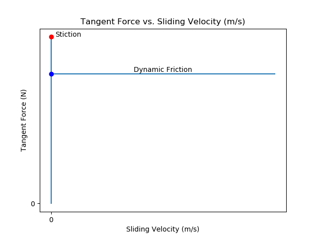
In idealized stiction, tangent force fₜ is equal and opposite to the pushing force fₚ up to the point where that force is sufficient to break stiction (the red dot in Figure 2). At that point, the tangent force immediately becomes a constant force based on the kinetic coefficient of friction. There are obvious discontinuities in this function which do not occur in reality, but this can be a useful approximation and can be implemented in this form using constraints that can be enabled and disabled discontinuously. However, here we are looking for a continuous model that can produce reasonable behavior using only unconstrained differential equations. With this model we can also capture the empirically-observed Stribeck effect where the friction force declines with increasing slip velocity until it reaches the kinetic friction level.
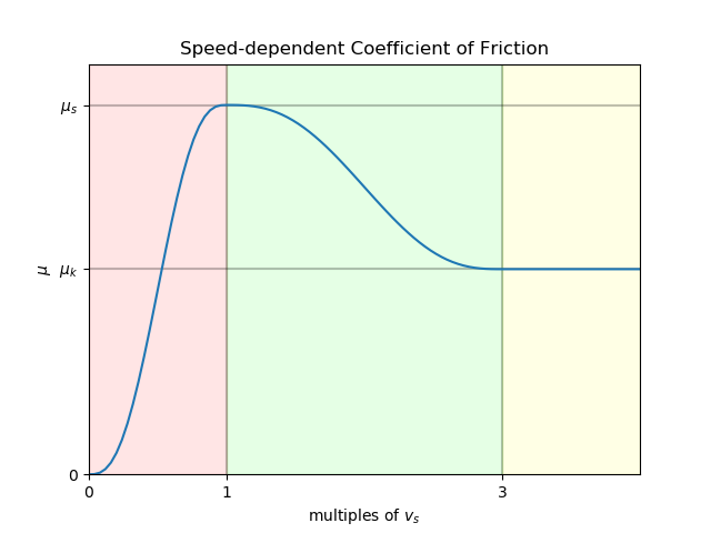
The Stribeck model is a variation of Coulomb friction, where the frictional (aka tangential) force is proportional to the normal force as: fₜ = μ⋅fₙ, In the Stribeck model, the coefficient of friction, μ, is replaced with a slip speed-dependent function: fₜ = μ(s)⋅fₙ, where s is a unitless multiple of a new parameter: slip tolerance (vₛ). Rather than modeling perfect stiction, it makes use of an allowable amount of relative motion to approximate stiction. When we refer to "relative motion", we refer specifically to the relative translational speed of two points Ac and Bc defined to instantly be located at contact point Co and moving with bodies A and B, respectively. The function, as illustrated in Figure 3, is a function of the unitless multiple of vₛ. The domain is divided into three intervals: